REVIEW 3 major objections 5 minor 34 references
The paper predicts that the weak decays Υ(3S)→B_c ℓν_ℓ have branching ratios up to 10^-9, the largest among bottomonium weak decays, and that the covariant light-front quark model provides reliable form factors for these transitions.
Reviewed by Pith at T0; open to challenge. T0 means a machine referee read the full paper against a public rubric. the ladder, T0–T4 →
T0 review · deepseek-v4-flash
2026-08-01 16:18 UTC pith:56IXZNSR
load-bearing objection CLFQM calculation worth a referee, but the headline Υ(3S)→B_c 10^-9 branching ratios ride on form factors the authors themselves label abnormal, so don't quote them as benchmarks yet. the 3 major comments →
The Upsilon(nS) to B_((c)) transition form factors and their applications to semileptonic and nonleptonic weak decays
The pith
A machine-rendered reading of the paper's core claim, the machinery that carries it, and where it could break.
Core claim
The authors claim that the CLFQM gives a reliable description of the Υ(nS)→B_(c) transition form factors, and that extrapolating these form factors from the spacelike to the timelike region via a double-pole parametrization yields definite predictions for the weak decays of bottomonia. They find that among all channels considered, Υ(3S)→B_c ℓν_ℓ has the largest branching ratios, of order 10^-9, driven by the narrow width of the Υ(3S) and a large vector form factor V(0)=2.22. For nonleptonic decays, Υ(3S)→B_c ρ and Υ(3S)→B_c D_s^(*) dominate, reaching 10^-10. They further report that the forward-backward asymmetry for Υ(3S)→B_(c) decays behaves anomalously compared with the other Υ(nS) states
What carries the argument
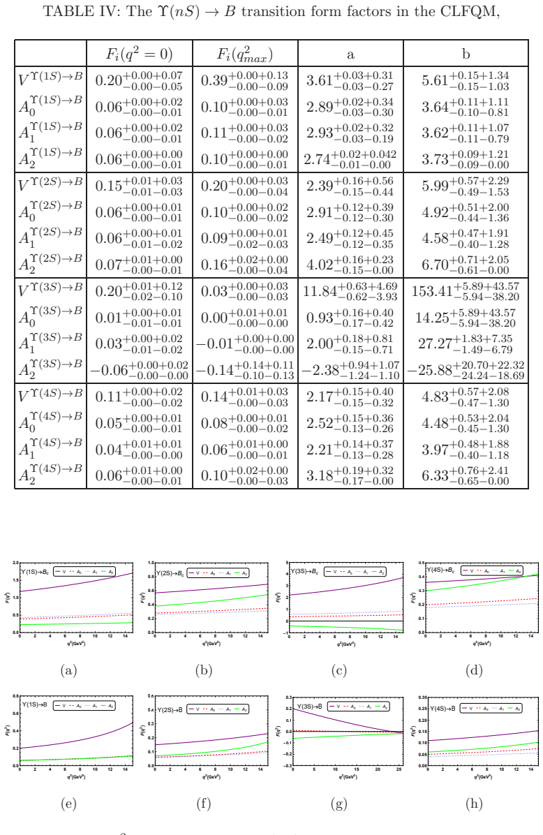
The central object is the set of BSW form factors V, A0, A1, A2 for the Υ(nS)→B_(c) transitions, computed in the covariant light-front quark model (CLFQM) and parametrized by the double-pole ansatz F(q^2)=F(0)/(1 - a q^2/m^2 + b q^4/m^4). These form factors feed the helicity amplitudes for semileptonic decays and the factorized amplitudes for nonleptonic decays, allowing branching ratios, forward-backward asymmetries, and longitudinal polarization fractions to be computed.
Load-bearing premise
The central predictions assume the CLFQM form factors computed at spacelike q^2 can be continued into the timelike region by a simple double-pole formula F(q^2)=F(0)/(1−a q^2/m^2+b q^4/m^4), with no additional singularities, and that the radial wavefunctions for the excited Υ(2S,3S,4S) states are accurate.
What would settle it
A measurement or lattice-QCD calculation of the Υ(3S)→B_c vector form factor at q^2=0 would settle the matter: if V(0) is substantially smaller than 2.22, the 10^-9 branching ratio prediction collapses. Also, a null result for Υ(3S)→B_c ℓν with an upper limit below 10^-10 would contradict the central claim.
If this is right
- If valid, Υ(3S)→B_c ℓν_ℓ decays become the most promising weak bottomonium channels, with branching ratios near 10^-9, detectable at future high-statistics experiments such as the HL-LHC.
- The predicted hierarchy Br(Υ(3S)→B_c M) > Br(Υ(2S)→B_c M) > Br(Υ(1S)→B_c M) for the same final meson M could be used to check the model's treatment of radially excited states.
- The lepton-flavor-universality ratios R_{Υ(nS)}^{B_c} would provide a clean test of the Standard Model if the branching ratios can be measured.
- Anomalous AFB behavior for Υ(3S)→B_(c) decays could serve as a sensitive probe of the form-factor shapes.
Where Pith is reading between the lines
- The prediction of Br(Υ(3S)→B_c ℓν) ≈ 10^-9 hinges on the unusually large CLFQM value V(0)=2.22 and the negative A2(0)=−0.42, which the authors themselves flag as anomalies; if these reflect a deficiency of the radial-excitation wavefunction rather than physics, the true rate could be considerably lower.
- The double-pole parametrization omits vector-meson pole terms; an alternative ansatz including such poles could shift the timelike form factors and alter the branching ratios, especially near q^2_max.
- The nonleptonic amplitudes use naive factorization with a single effective coefficient a1; for channels like Υ→B_c D_s^(*), QCD factorization or PQCD may introduce spectator/annihilation corrections that change the rates, so the comparison with PQCD results offers a direct experimental discriminator.
Editorial analysis
A structured set of objections, weighed in public.
Referee Report
Summary. The manuscript computes the Υ(nS) → B_{(c)} (n=1,2,3,4) transition form factors in the covariant light-front quark model (CLFQM), extrapolates them from spacelike q² to the physical timelike region with a double-pole ansatz (Eq. 35), and uses the resulting form factors to predict branching ratios for semileptonic Υ(nS) → B_{(c)} ℓν_ℓ and nonleptonic Υ(nS) → B_{(c)} M decays, together with forward-backward asymmetries and longitudinal polarization fractions. The headline results are Br(Υ(3S)→B_c ℓν) ≈ 5×10⁻⁹ and Br(Υ(3S)→B_c ρ, B_c D_s^(*)) up to 10⁻¹⁰, driven by the Υ(3S)→B_c vector form factor V(0)=2.22 and the anomalously negative A₂(0)=−0.42. The paper provides comparisons with BSW, NRQCD, BS, CCQM, PQCD and QCDF results and discusses the experimental prospects at HL-LHC and Belle-II.
Significance. If the CLFQM predictions were reliable, the paper would provide a useful, systematic survey of rare weak bottomonium decays and quantify discovery potentials for a challenging class of processes. Its strengths are the explicit form-factor formalism with analytical expressions in the appendices, the propagation of uncertainties from decay constants and widths, and the broad comparison with other models. However, the central numerical claims depend on two fragile ingredients: the shape parameters β are calibrated to the experimental leptonic decay constants, and, more importantly, the headline Υ(3S) rates are controlled by the same form factors that the paper itself calls "strange" and "abnormal" and that disagree strongly with NRQCD. In addition, the nonleptonic amplitudes contain an unspecified effective coefficient a₁, so those tables are not independently reproducible. The significance is therefore conditional on resolving these robustness issues.
major comments (3)
- [§III.A, Table III; §IV Summary] The central semileptonic claim, Br(Υ(3S)→B_c ℓν) ≈ 5×10⁻⁹, is driven by the Υ(3S)→B_c form factors V(0)=2.22 and A₂(0)=−0.42. These values are outliers relative to the 1S/2S/4S pattern and to NRQCD, which gives V(0)=1.25 and A₂(0)=0.29 (Table V). The manuscript itself acknowledges these results as "strange" and "abnormal" (Sec. III and Summary). Because the 3S radial wavefunction (Eq. 16) and the double-pole continuation (Eq. 35) are not independently validated, the headline branching ratio is not robust. Please provide a quantitative sensitivity test, e.g., repeating the Υ(3S)→B_c calculation with the NRQCD form factors, or using a dispersion-constrained parametrization, and discuss whether a negative A₂(0) is physically admissible.
- [§III.A, Eq. (35), Tables III and IV] The double-pole parametrization F(q²)=F(0)/(1−a q²/m² + b q⁴/m⁴) is fitted to spacelike points in −15 GeV² ≤ q² ≤ 0 and then continued to timelike q² up to about 16.6 GeV² for Υ(3S)→B_c and even further for Υ(3S)→B. The fit is purely numerical, with no vector-meson pole input, and for Υ(3S)→B some coefficients are extreme (e.g., a=11.84, b=153.41 for V in Table IV), indicating that the ansatz is poorly constrained. The paper should report the fit quality, the pole structure implied by the fitted a,b, and a comparison with an alternative extrapolation (e.g., z-expansion or a pole-dominated ansatz).
- [§III.D, Eqs. (30)–(31), Tables XI–XIV] Every nonleptonic branching ratio depends on the effective Wilson coefficient a₁, but no numerical value for a₁ is given anywhere in the paper. Equations (30) and (31) contain a₁, and all results in Tables XI–XIV use it, yet the input table (Table II) does not list it. The nonleptonic predictions are therefore not independently reproducible. Please specify the adopted a₁ value(s), their scale and scheme, and propagate the associated uncertainty.
minor comments (5)
- [References [4] and [5]] References [4] and [5] are identical; one of them is presumably a different paper. Please correct.
- [§III.D, text before Table XI] The text says the uncertainties come from the "lifetimes of Υ(nS)", but the numerical inputs are the total widths ΓΥ. Please use consistent terminology.
- [Figures 3 and 4] Both figures are garbled in the submitted PDF, with unreadable axis labels and legend text (e.g., "back, green and red solid" in Fig. 4 caption). Please regenerate the figures.
- [Throughout] There are numerous typos: "fowllowing", "Henna University Technology", "defination", "LUF" for "LFU", and in Eq. (4) the ISGW definition seems misaligned. A thorough proofread is needed.
- [§II.C, Eq. (27)] The effective Hamiltonian is written with V^*_{u(c)b}V_{qq'}, but the operator basis and the definition of a₁ should be spelled out more explicitly, including the treatment of color factors, so that Eq. (30) follows unambiguously.
Circularity Check
No circularity: CLFQM form factors are calibrated to leptonic decay constants and then applied to independent weak-decay observables; no predicted quantity is the fit input by construction.
full rationale
The derivation chain is: (1) experimental Υ(nS)→ℓ+ℓ− branching ratios enter Eq. (34) to extract fΥ; (2) these fΥ fix the phenomenological light-front shape parameters β in Eqs. (14)-(17); (3) β determines the Υ(nS)→B(c) form factors in Eqs. (C1)-(C4) at spacelike q²; (4) a double-pole parametrization (35) fitted to those spacelike form factors continues them to timelike q²; (5) helicity amplitudes (20)-(26) produce semileptonic branching ratios and Eqs. (30)-(33) nonleptonic ones. At no point is a predicted branching ratio algebraically identical to a fitted input. The fitted fΥ values are not the target observables; the weak decay rates depend on form factors, CKM elements, phase space and Υ total widths. The double-pole fit is an interpolation of the model's own form factors, not a fit to the decay rates. The paper's explicit caveats about the anomalous Υ(3S)→Bc form factors (V(0)=2.22, A2(0)=−0.42) and the differences from NRQCD/BSW are honesty about model uncertainty, not evidence that the result is equivalent to its inputs. Comparisons to prior work, including some by overlapping authors, are benchmarks rather than load-bearing premises. Thus no circular step satisfying the quoted-evidence standard is present.
Axiom & Free-Parameter Ledger
free parameters (5)
- β_Υ(1S), β_Υ(2S), β_Υ(3S), β_Υ(4S) (CLFQM shape parameters) =
1.289, 0.920, 0.808, 0.687 GeV
- β_B, β_Bc =
0.555, 1.058 GeV
- a, b double-pole coefficients for each form factor/transition =
Tables III-IV, e.g. V^{Υ(3S)→Bc}: a=2.91, b=4.71
- a1 (effective Wilson coefficient in nonleptonic amplitudes)
- constituent quark masses m_b, m_c, m_s, m_u/d =
4.8, 1.4, 0.37, 0.25 GeV
axioms (4)
- standard math Light-front contour integration and zero-mode replacement rules of Refs. [15,16] are valid for the Υ(nS)→B(c) vertex with radially excited states.
- domain assumption The double-pole ansatz F(q^2)=F(0)/(1-a q^2/m^2 + b q^4/m^4) remains valid for timelike q^2 up to (m_Υ−m_B(c))^2 and has no additional poles.
- domain assumption Gaussian (harmonic-oscillator) wavefunctions with nodal polynomials, Eqs. (14)-(17), describe radially excited Υ(2S,3S,4S) states.
- domain assumption Naive factorization for Υ→B(c)M: amplitudes factor into decay constant × form factor with a single a1; nonfactorizable/annihilation contributions are neglected.
read the original abstract
The semileptonic and nonleptonic decays of the $\Upsilon(nS)$ with $n=1,2,3,4$ are investigated within the covariant light-front quark model (CLFQM). Using the form factors of the transitions $\Upsilon(nS) \to B_{(c)}$ obtained from the CLFQM, we calculate the branching ratios of the decays $\Upsilon(nS)\to B_{(c)}\ell\nu_\ell$ and $\Upsilon(nS)\to B_{(c)}M$ with $\ell=e,\mu,\tau$ and $M$ referring to $\pi(\rho),K^{(*)},D^{(*)},D^{(*)}_s$. One can find that the branching ratios of the decays $\Upsilon(3S)\to B_c\ell\nu_\ell$ are the largest among those of considered semileptonic decays and can amount to $10^{-9}$; As to the nonleptonic decays, $\Upsilon(3S)\to B_c\rho$ and $\Upsilon(3S)\to B_cD^{(*)}_s$ have the largest branching ratios, which reach up to $10^{-10}$. Given the identification and detection efficiency of final states, searching for these weak decay modes should be fairly challenging in future experiments. The forward-backward asymmetry $A_{FB}$ and the longitudinal polarization fraction $f_L$ are also calculated for those semileptonic decays.
Figures



Reference graph
Works this paper leans on
-
[2]
In practice, we use the light- front decomposition of the Feynman loop momentum and integrate o ut the minus component through the contour method
γ5 (− ̸p2 + m2) ] .(10) The specific expressions for SΥB µν can be found in Appendix A. In practice, we use the light- front decomposition of the Feynman loop momentum and integrate o ut the minus component through the contour method. The specific rules for such integrat ion are displayed in Ap- pendix A. If the covariant vertex functions are not singular w...
2046
-
[3]
(γµ − γµγ5) (̸p′ 1 + m′
-
[4]
γ5 (− ̸p2 + m2) ] = −2iǫµναβ { p′α 1 P β (m′′ 1 − m′
-
[5]
+ p′α 1 qβ (m′′ 1 + m′ 1 − 2m2) + qαP βm′ 1 } + 1 W ′′ V (4p′ 1ν − 3qν − Pν) iǫµαβρp′α 1 qβP ρ +2gµν { m2 ( q2 − N ′ 1 − N ′′ 1 − m′2 1 − m′′2 1 ) − m′ 1 ( M ′′2 − N ′′ 1 − N2 − m′′2 1 − m2 2 ) −m′′ 1 ( M ′2 − N ′ 1 − N2 − m′2 1 − m2 2 ) − 2m′ 1m′′ 1m2 } +8p′ 1µp′ 1ν (m2 − m′
-
[6]
− 2 (Pµqν + qµPν + 2qµqν) m′ 1 + 2p′ 1µPν (m′ 1 − m′′ 1) +2p′ 1µqν (3m′ 1 − m′′ 1 − 2m2) + 2Pµp′ 1ν (m′ 1 + m′′
-
[7]
(A1) 20 Appendix B: Some specific rules under the p− intergration When preforming the integraion, we need to include the zero-mode c ontribution
+ 2qµp′ 1ν (3m′ 1 + m′′ 1 − 2m2) + 1 2W ′′ V (4p′ 1ν − 3qν − Pν) { 2p′ 1µ [ M ′2 + M ′′2 − q2 − 2N2 + 2 (m′ 1 − m2) (m′′ 1 + m2) ] +qµ [ q2 − 2M ′2 + N ′ 1 − N ′′ 1 + 2N2 − (m′ 1 + m′′ 1)2 + 2 (m′ 1 − m2)2 ] +Pµ [ q2 − N ′ 1 − N ′′ 1 − (m′ 1 + m′′ 1)2 ]} . (A1) 20 Appendix B: Some specific rules under the p− intergration When preforming the integraion, we ...
-
[8]
(x1m2 − x2m′′ 1 )] } , (C3) A0(q2) = M ′ + M ′′ 2M ′′ A1(q2) − M ′ − M ′′ 2M ′′ A2(q2) − q2 2M ′′ Nc 16π3 ∫ dx2d2p′ ⊥ h′ Υh′′ B(c) x2 ˆN ′ 1 ˆN ′′ 1 {2 (2x1 − 3) × (x2m′ 1 + x1m2) − 8 (m′ 1 − m2) × [ p′2 ⊥ q2 + 2 (p′ ⊥ · q⊥)2 q4 ] − [(14 − 12x1) m′ 1 −2m′′ 1 − (8 − 12x1) m2] p′ ⊥ · q⊥ q2 + 4 w′′ V ([ M ′2 + M ′′2 − q2 + 2 (m′ 1 − m2) (m′′ 1 + m2) ] × ( A(...
-
[9]
S. W. Herb et al. [E288], Phys. Rev. Lett. 39, 252 (1977). 23
1977
-
[10]
W. R. Innes et al. [E288], Phys. Rev. Lett. 39, 1240 (1977), [Erratum: Phys. Rev. Lett. 39, 1640 (1977)]
1977
-
[11]
Sanchis-Lozano, Z
M.A. Sanchis-Lozano, Z. Phys. C 62, 271 (1994)
1994
-
[13]
Y. Yang, J. Sun, Y. Guo, Q. Li, J. Huang and Q. Chang, Phys. L ett. B 751, 171-176 (2015) [arXiv:1701.04593 [hep-ph]]
Pith/arXiv arXiv 2015
-
[14]
J. Sun, Q. Li, Y. Yang, H. Li, Q. Chang and Z. Zhang, Phys. Re v. D 92, no.7, 074028 (2015) [arXiv:1610.06986 [hep-ph]]
Pith/arXiv arXiv 2015
-
[15]
T. Wang, Y. Jiang, H. Yuan, K. Chai, and G. L. Wang, J. Phys. G 44, no.4, 045004 (2017) [arXiv:1604.03298 [hep-ph]]
Pith/arXiv arXiv 2017
-
[17]
J. Sun, L. Chen, N. Wang, Q. Chang, J. Huang and Y. Yang, Adv . High Energy Phys. 2015, 691261 (2015) [arXiv:1610.06719 [hep-ph]]
Pith/arXiv arXiv 2015
-
[18]
J. Sun, L. Chen, N. Wang, J. Huang, Y. Yang and Q. Chang, J. Phys. G 42, no.10, 105005 (2015) [arXiv:1610.06723 [hep-ph]]
Pith/arXiv arXiv 2015
-
[19]
Chang, Y
Q. Chang, Y. Zhang and L. Han, Mod. Phys. Lett. A 31, no.38, 1650209 (2016)
2016
-
[20]
J. H. Sheng, F. Z. Zhou, Y. Y. Li and Y. G. Xu, Eur. Phys. J. C 85, no.3, 345 (2025)
2025
-
[21]
A. Cerri, V. V. Gligorov, S. Malvezzi, J. Martin Camalic h, J. Zupan, S. Akar, J. Alimena, B. C. Allanach, W. Altmannshofer and L. Anderlini, et al. CERN Yellow Rep. Monogr. 7, 867 (2019) [arXiv:1812.07638 [hep-ph]]
Pith/arXiv arXiv 2019
- [22]
-
[23]
H. Y. Cheng, C. K. Chua and C. W. Hwang, Phys. Rev. D 69, 074025 (2004) [arXiv:hep- ph/0310359 [hep-ph]]
arXiv 2004
-
[24]
Jaus, Phys
W. Jaus, Phys. Rev. D 60, 054026 (1999)
1999
-
[25]
Y. Sakaki, M. Tanaka, A. Tayduganov and R. Watanabe, Phy s. Rev. D 88, no.9, 094012 (2013) [arXiv:1309.0301 [hep-ph]]
Pith/arXiv arXiv 2013
-
[26]
G. Buchalla, A. J. Buras and M. E. Lautenbacher, Rev. Mod . Phys. 68, 1125-1144 (1996) [arXiv:hep-ph/9512380 [hep-ph]]
Pith/arXiv arXiv 1996
-
[27]
Navaset et al
S. Navaset et al. [Particle Data Group], Phys. Rev. D 110, 030001 (2024)
2024
-
[28]
D.Beˇ cirevi´ c, G.Duplanˇ ci´ c, B.Klajn, B.Meli´ c, F.Sanfilippo, Nucl. Phys. B 883, 306 (2014). arXiv:1312.2858[hep-ph]
Pith/arXiv arXiv 2014
-
[29]
T. W. Chiu, T. H. Hsieh, J. Y. Lee, P. H. Liu and H. J. Chang, Phys. Lett. B 624, 31 (2005) 24 [arXiv:hep-ph/0506266]
Pith/arXiv arXiv 2005
-
[30]
M. Wingate, C. T. H. Davies, A. Gray, G. P. Lepage and J. Sh igemitsu, Phys. Rev. Lett. 92, 162001 (2004) [arXiv:hep-ph/0311130]
Pith/arXiv arXiv 2004
-
[31]
Z. Q. Zhang, Z. J. Sun, Y. C. Zhao, Y. Y. Yang and Z. Y. Zhang , Eur. Phys. J. C 83, no.6, 477 (2023) [arXiv:2301.11107 [hep-ph]]
Pith/arXiv arXiv 2023
-
[32]
R. Dhir and R. C. Verma, Adv. High Energy Phys. 2013, 706543 (2013) [arXiv:0903.1201 [hep-ph]]
Pith/arXiv arXiv 2013
-
[33]
Chang, J
Q. Chang, J. Zhu, X. L. Wang, J. F. Sun and Y. L. Yang, J. Phy s. G 44, no.1, 015001 (2017)
2017
-
[34]
C. T. Tran, M. A. Ivanov, P. Santorelli and H. C. Tran, Chi n. Phys. C 49, no.1, 013111 (2025) [arXiv:2408.13776 [hep-ph]]
Pith/arXiv arXiv 2025
-
[35]
K. K. Sharma and R. C. Verma, Int. J. Mod. Phys. A 14, 937-946 (1999) [arXiv:hep- ph/9801202 [hep-ph]]
arXiv 1999
-
[36]
J. Sun, Y. Yang, J. Huang, G. Lu and Q. Chang, Nucl. Phys. B 911, 890-901 (2016) [arXiv:1709.10221 [hep-ph]]
Pith/arXiv arXiv 2016
-
[37]
J. Sun, Y. Yang, Q. Li, H. Li, Q. Chang and J. Huang, Phys. L ett. B 752, 322-328 (2016) [arXiv:1701.04597 [hep-ph]]. 25
Pith/arXiv arXiv 2016
discussion (0)
Sign in with ORCID, Apple, or X to comment. Anyone can read and Pith papers without signing in.