Adaptive Mamba Neural Operators

Zeyuan Song; Zheyu Jiang

REVIEW 3 major objections 4 minor 21 references

This paper claims that a new neural operator built from data-dependent Takenaka-Malmquist bases and state-space models reproduces adaptive Fourier decomposition and achieves the lowest relative L2 error across six PDE benchmarks.

Reviewed by Pith at T0; open to challenge. T0 means a machine referee read the full paper against a public rubric. the ladder, T0–T4 →

Challenge this review Re-run · record.json Download PDF Read on arXiv ↗

T0 review · deepseek-v4-flash

2026-08-01 16:15 UTC pith:EH4T6QXR

load-bearing objection The AMO architecture is new and the empirical work is real, but the paper's headline theory — that AMO provably performs AFD — is contradicted by its own equations: the implemented recurrence uses coefficients of the running state, while the convergence theorems require coefficients of a fixed target. the 3 major comments →

arxiv 2607.18043 v1 pith:EH4T6QXR submitted 2026-07-20 cs.LG cs.NAmath.APmath.NA

Adaptive Mamba Neural Operators

Zeyuan Song , Zheyu Jiang This is my paper

classification cs.LG cs.NAmath.APmath.NA

keywords neural operatorPDEsstate-space modelsMambaTakenaka-Malmquist systemadaptive Fourier decompositionBlack-Scholes equationoperator learning

verification ladder T0 review T1 audit T2 compute T3 formal T4 reserved

The pith

A machine-rendered reading of the paper's core claim, the machinery that carries it, and where it could break.

AMO is a neural operator for solving parametric PDEs on arbitrary meshes. It replaces the standard convolution-kernel view of state-space models with reproducing kernels built from Takenaka-Malmquist (TM) orthonormal bases, whose poles are predicted adaptively from the data. The authors' central claim is that this architecture reproduces adaptive Fourier decomposition (AFD): each block computes a TM coefficient, and the skip connection accumulates an AFD partial sum, so the network's output converges to the projection of the latent solution onto the selected TM space and inherits an explicit error bound. They further report that AMO beats state-of-the-art neural operators on six benchmark PDE families plus European option pricing, with an average relative L2 error reduction of about 28%. If both parts hold, AMO would be an operator-learning method that is simultaneously explainable, convergent in theory, and empirically ahead.

Core claim

The paper introduces an architecture in which a lifting layer compresses physical mesh tokens into M latent tokens; an MLP maps these tokens into an RKHS; a TM layer predicts a set of poles inside the unit disk and builds orthonormal Takenaka-Malmquist bases; and a bidirectional state-space model uses a transfer function set to the TM basis, making the block's zero-lag output the discrete inner product. The aggregation step is presented as exactly the AFD recursion, so after N blocks the latent representation is an N-term TM partial sum. The theory section states that if the SSM recovers the target coefficients, the latent approximation converges to the orthogonal projection of the latent so

What carries the argument

The central object is the Takenaka-Malmquist (TM) system: orthonormal rational bases B_i(z;a_{1:i}) built from adaptive poles a_i inside the unit disk, with each basis factor of the form sqrt(1-|a_i|^2)/(1-conj(a_i)z) times a Blaschke product over previous poles. The TM layer predicts the poles from the current token representation, the SSM's transfer function is set to B_i, and the block's output is the inner product of the current representation with B_i. The skip connection accumulates z_i plus the coefficient times B_i, which mirrors the AFD expansion of a signal in an orthonormal basis. This machinery turns the network into an adaptive rational spectral expansion whose basis adapts to t

Load-bearing premise

The load-bearing premise is that the coefficient read out by each SSM block equals the AFD coefficient of the fixed target s with respect to B_i, but the implemented recursion computes it against the running aggregate z_i; the two agree only before the first update, so if that identification fails, the convergence theorem's premise fails.

What would settle it

A two-term calculation settles it: set s = c1 B1 + c2 B2 with orthonormal B1, B2 and nonzero c1, c2. Following the implemented update, the first block gives the coefficient c1 and sets z2 = c1 B1; the second block then computes the coefficient of z2 against B2, which is 0, not c2. Running this small example shows whether the recursion actually produces AFD coefficients of s or of the evolving aggregate.

Watch this falsifier — get emailed when new claim-graph text bears on it.

If this is right

Because the architecture is an AFD-style accumulation, each additional processing block extends the TM partial sum, so the latent error is expected to decrease as the number of blocks and poles grows, barring optimization error.
The learned pole positions are interpretable: poles clustering near the unit circle correspond to boundary-localized or singular features, while interior poles track volume-distributed nonlinear reactions, providing a built-in diagnostic.
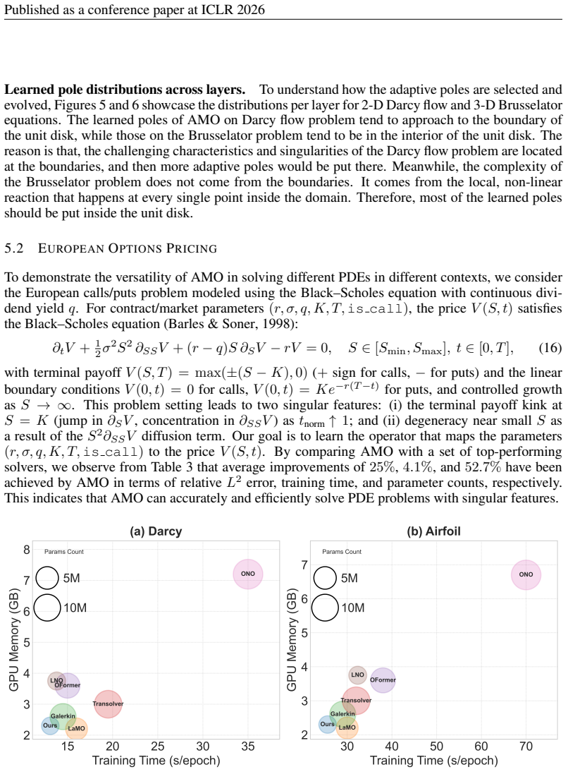
Orthonormal TM bases avoid explicit orthogonalization, which the paper reports saves roughly 2.7x training time and 3x GPU memory relative to an orthogonal-attention-based solver, while complexity stays approximately linear in the number of mesh points.
The reported empirical gains (relative L2 reductions from 11.5% to 51.2% across six benchmarks, plus gains on option pricing and a real glove-displacement dataset) indicate the design transfers across regular grids, structured meshes, point clouds, and noisy experimental data.

Where Pith is reading between the lines

These are editorial extensions of the paper, not claims the author makes directly.

A reader's inference: the proof's coefficient identification deserves scrutiny. Equation (11) reads out the inner product of the running aggregate z_i with B_i, while Lemma D.3 needs the inner product of the fixed target s with B_i; these two quantities differ after the first update, so the claimed 'exact AFD' status is stronger than the current derivation supports.
If the mismatch were patched by making each block recompute against the original target representation, the convergence theorem would align with the update rule; the empirical comparisons would likely survive unchanged, making the architecture's practical value largely independent of the theoretical label.
The pole-location visualizations could be turned into a predictive diagnostic: train once on a PDE family and use the pole distribution as a signature that distinguishes boundary-dominated from interior-reaction-dominated regimes, potentially guiding mesh refinement or pole-count selection on new instances.

Editorial analysis

A structured set of objections, weighed in public.

Desk editor's note, referee report, simulated authors' rebuttal, and a circularity audit.

Desk Editor's Note

The AMO architecture is new and the empirical work is real, but the paper's headline theory — that AMO provably performs AFD — is contradicted by its own equations: the implemented recurrence uses coefficients of the running state, while the convergence theorems require coefficients of a fixed target.

read the letter

Two things to know. First, the AMO architecture is new — TM bases built from learned poles, used as SSM transfer functions in the frequency domain — and the empirical program is serious: six benchmarks plus option pricing, ablations on adaptive versus static kernels, orthogonality, SSM choice, and a nice pole-distribution analysis. Second, the paper's headline theory is wrong, and the paper contradicts itself to show it. Section 3.2's Eqs. (11)-(12) compute ⟨z_i, B_i⟩, the inner product of the running latent state against the TM basis, and aggregate as z_{i+1} = z_i + ⟨z_i, B_i⟩B_i. Section 4 even writes z_{i+1} = Σ_{k≤i} ⟨z_k, B_k⟩B_k and calls this 'equivalent to the AFD operation.' It isn't. AFD expands a fixed target s as Σ ⟨s, B_k⟩B_k. The convergence machinery in Appendix D (Lemma D.3, Theorem D.4, D.13) assumes exactly those target coefficients c*_i = ⟨s, B_i⟩, and Proposition D.14 then says the SSM block actually computes ⟨z_i, B_i⟩ — its proof licenses this by applying Lemma D.3 'with z_i in place of s.' That substitution is the whole problem: the two coefficient types agree only when z_i = s, which is false after the first update.

The consequence is concrete. For an orthonormal TM system, the implemented update doubles each processed coefficient: after N blocks the latent is 2Σ_{i≤N} a_i B_i + Σ_{i>N} a_i B_i, so its norm heads to 2‖s‖, not ‖s‖, and it does not converge to s or its projection. In the appendix's own initial condition (z_1 = 0), the recurrence outputs zero identically. So the convergence guarantees advertised in the abstract and contribution 1 are proofs about a different algorithm than the one trained and tested.

Credits where they are due. The adaptive-pole mechanism is well motivated; using Blaschke products as transfer functions inside a Mamba block is a clean idea; the ablations are informative. The reproducibility statement and code link are in the right spirit. The claimed 28% average relative-L2 gain is plausible, but Table 1 has no error bars or seed variance, so the margin over LaMO is unverified. Minor issues: the discrete inner product omits complex conjugation; the quadrature and learning rates (Lemma D.9, Assumption D.8) are assumed, not derived; and no constraint is specified for keeping the MLP's poles inside the unit disk.

Who gets value: anyone working on SSM-based or spectral neural operators can learn from the architecture, and the paper is a good reading-group case study in checking that theory matches implementation. The convergence theory should not be cited.

Recommendation: engage with it. Send it to a serious referee with an explicit request to reconcile Proposition D.14 with Theorem D.4. If the authors fix the recurrence (e.g., a residual update) or retract the AFD-convergence claim and present AMO as an empirically motivated architecture, the paper is defensible. As written, the headline theory should not be accepted. I'd call it major revision or reject, with the architecture worth salvaging.

Referee Report

3 major / 4 minor

Summary. The paper proposes Adaptive Mamba Neural Operators (AMO), a neural operator architecture that integrates Takenaka–Malmquist (TM) systems and state-space models (SSMs) in the frequency domain. The central claim is that AMO performs adaptive Fourier decomposition (AFD) approximation of PDE solutions, providing explainability and rigorous convergence guarantees. The paper reports state-of-the-art relative L2 errors on six benchmark PDE problems plus an option-pricing problem, along with ablation studies on adaptive versus static poles, orthogonality of kernels, and choice of SSM direction. The main theoretical contribution is presented in Section 4 and Appendix D, where the authors claim equivalence between the AMO recurrence and AFD and prove convergence to the orthogonal projection of the target onto the TM model space.

Significance. If the AFD-equivalence and convergence claims were correct, this would be a significant contribution: a neural operator with an orthonormal, adaptive spectral basis, theoretical convergence guarantees, and strong empirical accuracy across regular and irregular geometries. The paper also provides code and a detailed experimental setup, which is commendable. However, the central theoretical claim is not supported by the derivation. The architecture computes coefficients of the running aggregate z_i, not of the fixed target s, while the convergence theorems assume the latter. This breaks the advertised explainability and convergence guarantees, reducing the paper's contribution to a set of empirical results with a plausible but unproven connection to AFD. The empirical performance itself is not questioned here, but the theoretical foundation, which is a key stated contribution, is invalid as written.

major comments (3)

[Section 3.2, Eqs. (10)–(12), vs. Appendix D.2, Eqs. (23)–(24) and Theorem D.4] The implemented update (Eq. (12)) is z_{i+1} = z_i + ⟨z_i, B_i⟩ B_i, because the SSM input is the current latent z_i (Eq. (11)). In contrast, Appendix D defines z_{i+1} = z_i + ĉ_i B_i where ĉ_i estimates c*_i = ⟨s, B_i⟩_H for a fixed target s (Eq. (24)). These coincide only if z_i = s, which is false after the first update and is false from the start since z_1 is the output of R∘P, not s. Consequently, Theorem D.4, which assumes 'AMO recovers the exact coefficients c*_i,' proves convergence for a different algorithm than the one described. For an orthonormal TM system, the implemented recursion doubles the processed coefficients; the N-block output does not converge to s or to Π_{K_B} s. This directly invalidates the paper's claim that AMO provably performs AFD approximation.
[Appendix D.7, Proposition D.14 vs. Lemma D.3] Proposition D.14 explicitly states that the i-th SSM block computes bc_i ≈ ⟨z_i, B_i⟩_H, applying Lemma D.3 with z_i in place of s. But Lemma D.3 and Theorem D.4 require bc_i ≈ ⟨s, B_i⟩_H. The paper never bridges this gap, and the two coefficient sequences are generally unrelated. This is not a minor notational issue: the proof of the end-to-end convergence theorem (Theorem D.13) rests entirely on the unstated identification of ⟨z_i, B_i⟩ with ⟨s, B_i⟩. Since Proposition D.14 confirms the former, the theoretical results in Appendix D analyze a recurrence that the architecture does not implement.
[Section 4, 'Connections to AFD theory'] The claim that 'the output of Equation 12 z_{i+1} is equivalent to the AFD operation, i.e., z_{i+1} = Σ_{k=1}^i ⟨z_k, B_k⟩ B_k' is not a statement of AFD. AFD expands a fixed signal s as Σ ⟨s, B_k⟩ B_k; the running coefficients ⟨z_k, B_k⟩ do not yield an AFD partial sum of s. The same issue propagates to Eq. (13) and to the interpretation of the output as 'exactly matches with AFD operation.' The theoretical contribution stated in the Introduction ('prove that AMO performs AFD approximation of PDE solutions') is therefore unsupported.

minor comments (4)

[Throughout] The paper label 'LAMO' (e.g., Table 1) and 'LaMO' (e.g., Section 1) are used inconsistently for the same baseline. Please standardize.
[Eq. (15)] The denominator in the relative L2 error formula is written '||G(a_i)|L2'; the norm bars are incomplete. Should be ||G(a_i)||_{L2}.
[Introduction and Conclusion] There are typos: 'frenquency' (Section 1) and 'oepration' (Section 6). These should be corrected.
[Section 3.2, after Eq. (12)] The formula 'z_2 = S_1(z_1, ĉ_2[0], B_1) = ĉ_2[0]⊙B_1' is inconsistent with the general recurrence z_{i+1}=z_i+... for i>1; either the i=1 base case should be included in the general rule or the notation for ĉ_2[0] should be clarified.

Circularity Check

2 steps flagged

AMO's convergence theorem assumes the target coefficients it never computes: Eq. (11) defines the block output as ⟨z_i,B_i⟩, while Theorem D.4 requires ⟨s,B_i⟩.

specific steps

self definitional [Section 3.2, Eqs. (11)-(12); Section 4, 'Connections to AFD theory']
"ˆzi+1[0] = ... = ⟨z_i,B_i⟩ ... zi+1 = S_i(zi, ˆzi+1[0],B_i) = z_i + (ˆzi+1[0]⊙B_i). ... Thus, the output of Equation 12 z_{i+1}, is equivalent to the AFD operation, i.e., z_{i+1} = Σ_{k=1}^i⟨z_k,B_k⟩B_k."

Eq. (11) defines the coefficient as an inner product of the running aggregate z_i with B_i, and Eq. (12) builds z_{i+1} by adding that coefficient times B_i. Section 4 then names this recurrence 'the AFD operation.' But the AFD convergence theorem invoked by the paper is for the fixed-target coefficients c_i^* = ⟨s,B_i⟩_H. No step shows ⟨z_i,B_i⟩ = ⟨s,B_i⟩; with Eq. (12), z_{i+1} = Σ_{k≤i}⟨z_k,B_k⟩B_k, so already z_2 = ⟨z_1,B_1⟩B_1 and ⟨z_2,B_2⟩ = 0, not ⟨s,B_2⟩. The claimed convergence to s is therefore not a derived consequence; it is the same identification being assumed, and the theory reduces to standard Hilbert-space expansion of an assumed coefficient sequence.
fitted input called prediction [Appendix D.2, Lemma D.3; Appendix D.7, Proposition D.14; Theorem D.4]
"Lemma D.3. ... If the discrete inner product used by AMO is a consistent quadrature for ⟨·,·⟩_H on the class {s} ∪ {B_i}, then bci → ⟨s,B_i⟩_H = c_i^*. ... Proposition D.14. With H_i(e^{iω}) = B_i(e^{iω}), the i-th SSM block computes bci ≈ ⟨z_i,B_i⟩_H."

Lemma D.3 obtains bci as the inner product of the fixed target s with B_i, by taking the block's input spectrum to be s. Proposition D.14 acknowledges that the implemented block computes the inner product of the current aggregate z_i with B_i. These coincide only if z_i = s, which Eq. (12) does not preserve. The computed quantity ⟨z_i,B_i⟩ is therefore renamed as the target AFD coefficient c_i^*, and Theorem D.4's premise ('if AMO recovers the exact coefficients c_i^*') is exactly the unproved identification the architecture does not supply. The running-state inner product is presented as the predicted fixed-target coefficient.

full rationale

The empirical part is not circular: Tables 1-5 compare AMO against external baselines on public benchmarks (plasticity, elasticity, airfoil, pipe, N-S, Darcy, options, DIC), and those accuracy gains do not depend on the AFD theorem. The circularity is confined to the theoretical claim that 'AMO performs AFD approximation of PDE solutions.' Section 4 defines the output of Eq. (12) as 'equivalent to the AFD operation,' i.e., z_{i+1} = Σ⟨z_k,B_k⟩B_k, then invokes the AFD convergence theorem whose coefficients are ⟨s,B_i⟩ for a fixed target s (D.2, D.4). Eq. (11) and Prop. D.14 fix the actual block coefficient as ⟨z_i,B_i⟩. Under Eq. (12)'s aggregation, after the first block z_2 = ⟨z_1,B_1⟩B_1, so ⟨z_2,B_2⟩ = 0; the subsequent coefficients are not the target coefficients ⟨s,B_i⟩. Thus Theorem D.4 proves a statement about an assumed coefficient sequence, not about the implemented recurrence. The only link between the two is the definitional assertion that the recurrence is AFD. This is a self-definitional reduction: the conclusion 'AMO performs AFD approximation' is built into the naming of the recurrence, while the mathematical content is the standard Hilbert-space expansion of an assumed target coefficient. Because the central theoretical contribution reduces by construction/assumption, score 7. No self-citation chain is involved; no external benchmark is used as a circular input.

Axiom & Free-Parameter Ledger

3 free parameters · 5 axioms · 0 invented entities

The central theoretical claims rest on five substantive assumptions, several of which are not established for the implemented architecture. The most damaging is the unstated identification of the SSM output ⟨z_i,B_i⟩ with the AFD coefficient ⟨s,B_i⟩ of the fixed target. The paper's convergence theorems are conditional on exactly the quantities that the network is supposed to learn, and on quadrature/ERM assumptions that are asserted but not proved.

free parameters (3)

learned poles a_1:i = learned; specific values not reported
Construct the TM bases (Eq. 6); the adaptivity of these poles is the paper's core mechanism and is trained by a small MLP per layer.
network weights (MLP, SSM, P, Q) = learned; only total sizes reported (e.g., AMO 1.21M params for options)
All approximation power comes from trained parameters; no per-component audit is given.
architectural hyperparameters = M=64 tokens, D=128 width, 4 blocks, 32 poles, SSM state size 16
Chosen by hand; ablation only varies pole count. These values affect every reported result.

axioms (5)

domain assumption Assumption D.1: H is an RKHS on the unit disk with normalized reproducing kernels e_a and TM system {B_i} orthonormal, spanning K_B.
This is true for classical Hardy spaces but is assumed for the paper's abstract RKHS H and for PDE solution manifolds mapped by R; no construction is given.
ad hoc to paper The discrete inner product over M/Ñ grid points is a consistent quadrature for ⟨·,·⟩_H on {s} ∪ {B_i}.
Lemma D.9 asserts this via 'standard quadrature consistency' but provides no quadrature error bounds for the specific finite-token representation used in AMO. The inner product in the main text also omits complex conjugation.
ad hoc to paper Assumption D.8: the learned coefficients satisfy E[|ĉ_i−c_i^★|]=O(sqrt(d_eff/m)) under sub-Gaussian noise.
A generic ERM bound assumed without proof for the AMO architecture; it is exactly the quantity that would make the convergence theorem non-vacuous.
ad hoc to paper The MLP-chosen poles define K_B and the target s lies in K_B (Theorem D.13, condition 1).
Needed for the error to vanish as N→∞; otherwise only convergence to Π_{K_B}s, not to s, is guaranteed.
domain assumption R maps finite encoded tokens to functions in H that satisfy pointwise evaluation and the inner-product identities.
The implementation is MLP(z0) (Eq. 4); the theory treats z_i as continuous functions in H. Compatibility is not shown.

pith-pipeline@v1.3.0-alltime-deepseek · 18316 in / 15739 out tokens · 160929 ms · 2026-08-01T16:15:02.147771+00:00 · methodology

0 comments

read the original abstract

Accurately solving partial differential equations (PDEs) on arbitrary geometries and a variety of meshes is an important task in science and engineering applications. In this paper, we propose Adaptive Mamba Neural Operators (AMO), which integrates reproducing kernels for state-space models (SSMs) rather than the kernel integral formulation of SSMs. This is achieved by constructing Takenaka-Malmquist systems for the PDEs. AMO offers new representations that align well with the adaptive Fourier decomposition (AFD) theory and can approximate the solution manifold of PDEs on a wide range of geometries and meshes. In several challenging benchmark PDE problems in the fields of fluid physics, solid physics, and finance on point clouds, structured meshes, regular grids, and irregular domains, AMO consistently outperforms state-of-the-art solvers in terms of relative $L^2$ error. Overall, this work presents a new paradigm for designing explainable neural operator frameworks.

Figures

Figures reproduced from arXiv: 2607.18043 by Zeyuan Song, Zheyu Jiang.

**Figure 2.** Figure 2: Contribution of three SSMs across seven benchmark datasets. Note that we do not apply [PITH_FULL_IMAGE:figures/full_fig_p010_2.png] view at source ↗

**Figure 3.** Figure 3: Phase error of solutions predicted by LaMO. [PITH_FULL_IMAGE:figures/full_fig_p014_3.png] view at source ↗

**Figure 4.** Figure 4: The predicted results produced by LaMO compared to the ground truth. [PITH_FULL_IMAGE:figures/full_fig_p015_4.png] view at source ↗

**Figure 5.** Figure 5: Learned poles distribution for the 2-D Darcy flow equation. [PITH_FULL_IMAGE:figures/full_fig_p016_5.png] view at source ↗

**Figure 6.** Figure 6: Learned poles distribution for the 3-D Brusselator equation. [PITH_FULL_IMAGE:figures/full_fig_p017_6.png] view at source ↗

discussion (0)

Reference graph

Works this paper leans on

21 extracted references · 13 linked inside Pith

[3]

Efficiently modeling long sequences with structured state spaces.arXiv preprint arXiv:2111.00396,

Albert Gu, Karan Goel, and Christopher R ´e. Efficiently modeling long sequences with structured state spaces.arXiv preprint arXiv:2111.00396,

Pith/arXiv arXiv
[5]

To clarify, here we give a brief overview of the visualization results: The distribution of selected poles for the 2-D Darcy flow problem is shown in Figures 5 and 6, respectively. We observe that, across the layers, the learned poles of AMO on Darcy flow problem tend to ap- proach to the boundary of the unit disk, while those on the Brusselator problem t...

2026
[6]

Transformer for partial differential equations’ operator learning.arXiv preprint arXiv:2205.13671,

Zijie Li, Kazem Meidani, and Amir Barati Farimani. Transformer for partial differential equations’ operator learning.arXiv preprint arXiv:2205.13671,

Pith/arXiv arXiv
[7]

Fourier neural operator for parametric partial differential equations.arXiv preprint arXiv:2010.08895,

Zongyi Li, Nikola Kovachki, Kamyar Azizzadenesheli, Burigede Liu, Kaushik Bhattacharya, An- drew Stuart, and Anima Anandkumar. Fourier neural operator for parametric partial differential equations.arXiv preprint arXiv:2010.08895,

Pith/arXiv arXiv 2010
[8]

Beyond regular grids: Fourier-based neural operators on arbitrary do- mains.arXiv preprint arXiv:2305.19663,

Levi Lingsch, Mike Y Michelis, Emmanuel De B ´ezenac, Sirani M Perera, Robert K Katzschmann, and Siddhartha Mishra. Beyond regular grids: Fourier-based neural operators on arbitrary do- mains.arXiv preprint arXiv:2305.19663,

arXiv
[9]

Decoupled weight decay regularization.arXiv preprint arXiv:1711.05101,

Ilya Loshchilov and Frank Hutter. Decoupled weight decay regularization.arXiv preprint arXiv:1711.05101,

Pith/arXiv arXiv
[12]

Factorized fourier neural operators.arXiv preprint arXiv:2111.13802,

Alasdair Tran, Alexander Mathews, Lexing Xie, and Cheng Soon Ong. Factorized fourier neural operators.arXiv preprint arXiv:2111.13802,

Pith/arXiv arXiv
[13]

Solving high- dimensional PDEs with latent spectral models.arXiv preprint arXiv:2301.12664,

Haixu Wu, Tengge Hu, Huakun Luo, Jianmin Wang, and Mingsheng Long. Solving high- dimensional PDEs with latent spectral models.arXiv preprint arXiv:2301.12664,

Pith/arXiv arXiv
[14]

Transolver: A fast transformer solver for pdes on general geometries.arXiv preprint arXiv:2402.02366,

Haixu Wu, Huakun Luo, Haowen Wang, Jianmin Wang, and Mingsheng Long. Transolver: A fast transformer solver for pdes on general geometries.arXiv preprint arXiv:2402.02366,

Pith/arXiv arXiv
[15]

Coupled multiwavelet neural operator learning for coupled partial dif- ferential equations.arXiv preprint arXiv:2303.02304, 2023a

Xiongye Xiao, Defu Cao, Ruochen Yang, Gaurav Gupta, Gengshuo Liu, Chenzhong Yin, Radu Balan, and Paul Bogdan. Coupled multiwavelet neural operator learning for coupled partial dif- ferential equations.arXiv preprint arXiv:2303.02304, 2023a. Zipeng Xiao, Zhongkai Hao, Bokai Lin, Zhijie Deng, and Hang Su. Improved operator learning by orthogonal attention.a...

Pith/arXiv arXiv
[16]

12 Published as a conference paper at ICLR 2026 A NOTATIONLIST aParameter function (input) ˆuN,θ Output of AMO withNblocks and parametersθ NNumber of processing blocks Ns Number of input physical tokens MNumber of encoded latent tokens (M≪N s) Dembed Embedding dimension of latent tokens xphys Input physical features gphys Positional embedding of coordinat...

2026
[20]

For 38, use the mean-value theorem onx7→ √1−xwithx=|a| 2,|b| 2 and||a| 2 − |b|2| ≤ |a−b|(|a|+|b|)≤2|a−b|

D.5 STABILITY TO POLE PERTURBATIONS Lemma D.11.Fora, b∈Dandz∈D, 1 1− az − 1 1− bz ≤ |a−b| (1− |a|)(1− |b|),(37) p 1− |a|2 − p 1− |b|2 ≤ |a−b|p 1−max{|a|,|b|} 2 ,(38) and forF(z;a) = z−a 1− az , |F(z;a)−F(z;b)| ≤ 4|a−b| (1− |a|)(1− |b|),|F(z;a)| ≤1.(39) Proof.For 37, 1 1− az − 1 1− bz = (a− b)z (1− az)(1− bz) , and|1− az| ≥1− |a||z| ≥1− |a|,|z| ≤1, yieldin...

2026
[21]

Hence, by Lemma D.2, afterNblocks zN+1 = NX i=1 bci Bi,ˆu N,θ =Q(z N+1 ).(42) Proof.The coefficient claim follows from Lemma D.3 applied toz i in place ofs

D.7 CONNECTION OFSSMTO CORRELATION ANDAMOOUTPUT Proposition D.14.WithH i(eiω) = Bi(eiω), thei-th SSM block computesbci ≈ ⟨zi,B i⟩H. Hence, by Lemma D.2, afterNblocks zN+1 = NX i=1 bci Bi,ˆu N,θ =Q(z N+1 ).(42) Proof.The coefficient claim follows from Lemma D.3 applied toz i in place ofs. The aggregation identity is Lemma D.2. The last equality is the defi...

2026
[28]

Remark.No greedy or maximal selection is used

The bound 29 follows from Lipschitz continuity ofQ: ∥u⋆ − Q(sN )∥=∥Q(s)− Q(sN )∥ ≤LQ∥s−s N ∥ ≤LQ ∥s−Π KB s∥+∥Π KB s−s N ∥ . Remark.No greedy or maximal selection is used. The MLP-generated poles determineK B; AMO converges toΠ KB s, and toswhenevers∈K B. D.3 BESTN-TERM ERROR AND RATES WITHOUT GREEDY SELECTION Definition D.5.LetD:={B i(·;a 1:i) :a 1:i ∈D i...

2026
[35]

Proof.Apply Theorem D.6 to bound the latentH-error

(Iff, gare analytic in an annulus around the unit circle, one gets exponential rates; under Sobolev regularity, algebraic rates.) 19 Published as a conference paper at ICLR 2026 Theorem D.10.Under Assumptions D.1 and D.8 and Lemma D.9, the AMO output afterNblocks and ˜Ngrid points satisfies ∥u⋆ −ˆuN,θ ∥ ≤L Q EN (s) + ∆pole(N) + NX i=1 |bci −c ⋆ i |2 1/2 +...

2026
[2012]

U-no: U-shaped neural oper- ators.arXiv preprint arXiv:2204.11127,

Md Ashiqur Rahman, Zachary E Ross, and Kamyar Azizzadenesheli. U-no: U-shaped neural oper- ators.arXiv preprint arXiv:2204.11127,

Pith/arXiv arXiv
[2021]

Adaptive Fourier neural operators: Efficient token mixers for transformers.arXiv preprint arXiv:2111.13587,

John Guibas, Morteza Mardani, Zongyi Li, Andrew Tao, Anima Anandkumar, and Bryan Catan- zaro. Adaptive Fourier neural operators: Efficient token mixers for transformers.arXiv preprint arXiv:2111.13587,

Pith/arXiv arXiv
[2022]

State-space models are accurate and efficient neural operators for dynamical systems

Zheyuan Hu, Nazanin Ahmadi Daryakenari, Qianli Shen, Kenji Kawaguchi, and George Em Kar- niadakis. State-space models are accurate and efficient neural operators for dynamical systems. arXiv preprint arXiv:2409.03231,

Pith/arXiv arXiv
[2023]

Mamba: Linear-time sequence modeling with selective state spaces.arXiv preprint arXiv:2312.00752,

Albert Gu and Tri Dao. Mamba: Linear-time sequence modeling with selective state spaces.arXiv preprint arXiv:2312.00752,

Pith/arXiv arXiv
[2024]

Mamba neural operator: Who wins? transformers vs

Chun-Wun Cheng, Jiahao Huang, Yi Zhang, Guang Yang, Carola-Bibiane Sch¨onlieb, and Angelica I Aviles-Rivero. Mamba neural operator: Who wins? transformers vs. state-space models for pdes. arXiv preprint arXiv:2410.02113,

arXiv
[2025]

URL https://arxiv.org/abs/2502.02414. 11 Published as a conference paper at ICLR 2026 Rom N Parnichkun, Stefano Massaroli, Alessandro Moro, Jimmy TH Smith, Ramin Hasani, Mathias Lechner, Qi An, Christopher R ´e, Hajime Asama, Stefano Ermon, et al. State-free inference of state-space models: The transfer function approach.arXiv preprint arXiv:2405.06147,

Pith/arXiv arXiv 2026

[1] [3]

Efficiently modeling long sequences with structured state spaces.arXiv preprint arXiv:2111.00396,

Albert Gu, Karan Goel, and Christopher R ´e. Efficiently modeling long sequences with structured state spaces.arXiv preprint arXiv:2111.00396,

Pith/arXiv arXiv

[2] [5]

To clarify, here we give a brief overview of the visualization results: The distribution of selected poles for the 2-D Darcy flow problem is shown in Figures 5 and 6, respectively. We observe that, across the layers, the learned poles of AMO on Darcy flow problem tend to ap- proach to the boundary of the unit disk, while those on the Brusselator problem t...

2026

[3] [6]

Transformer for partial differential equations’ operator learning.arXiv preprint arXiv:2205.13671,

Zijie Li, Kazem Meidani, and Amir Barati Farimani. Transformer for partial differential equations’ operator learning.arXiv preprint arXiv:2205.13671,

Pith/arXiv arXiv

[4] [7]

Fourier neural operator for parametric partial differential equations.arXiv preprint arXiv:2010.08895,

Zongyi Li, Nikola Kovachki, Kamyar Azizzadenesheli, Burigede Liu, Kaushik Bhattacharya, An- drew Stuart, and Anima Anandkumar. Fourier neural operator for parametric partial differential equations.arXiv preprint arXiv:2010.08895,

Pith/arXiv arXiv 2010

[5] [8]

Beyond regular grids: Fourier-based neural operators on arbitrary do- mains.arXiv preprint arXiv:2305.19663,

Levi Lingsch, Mike Y Michelis, Emmanuel De B ´ezenac, Sirani M Perera, Robert K Katzschmann, and Siddhartha Mishra. Beyond regular grids: Fourier-based neural operators on arbitrary do- mains.arXiv preprint arXiv:2305.19663,

arXiv

[6] [9]

Decoupled weight decay regularization.arXiv preprint arXiv:1711.05101,

Ilya Loshchilov and Frank Hutter. Decoupled weight decay regularization.arXiv preprint arXiv:1711.05101,

Pith/arXiv arXiv

[7] [12]

Factorized fourier neural operators.arXiv preprint arXiv:2111.13802,

Alasdair Tran, Alexander Mathews, Lexing Xie, and Cheng Soon Ong. Factorized fourier neural operators.arXiv preprint arXiv:2111.13802,

Pith/arXiv arXiv

[8] [13]

Solving high- dimensional PDEs with latent spectral models.arXiv preprint arXiv:2301.12664,

Haixu Wu, Tengge Hu, Huakun Luo, Jianmin Wang, and Mingsheng Long. Solving high- dimensional PDEs with latent spectral models.arXiv preprint arXiv:2301.12664,

Pith/arXiv arXiv

[9] [14]

Transolver: A fast transformer solver for pdes on general geometries.arXiv preprint arXiv:2402.02366,

Haixu Wu, Huakun Luo, Haowen Wang, Jianmin Wang, and Mingsheng Long. Transolver: A fast transformer solver for pdes on general geometries.arXiv preprint arXiv:2402.02366,

Pith/arXiv arXiv

[10] [15]

Coupled multiwavelet neural operator learning for coupled partial dif- ferential equations.arXiv preprint arXiv:2303.02304, 2023a

Xiongye Xiao, Defu Cao, Ruochen Yang, Gaurav Gupta, Gengshuo Liu, Chenzhong Yin, Radu Balan, and Paul Bogdan. Coupled multiwavelet neural operator learning for coupled partial dif- ferential equations.arXiv preprint arXiv:2303.02304, 2023a. Zipeng Xiao, Zhongkai Hao, Bokai Lin, Zhijie Deng, and Hang Su. Improved operator learning by orthogonal attention.a...

Pith/arXiv arXiv

[11] [16]

12 Published as a conference paper at ICLR 2026 A NOTATIONLIST aParameter function (input) ˆuN,θ Output of AMO withNblocks and parametersθ NNumber of processing blocks Ns Number of input physical tokens MNumber of encoded latent tokens (M≪N s) Dembed Embedding dimension of latent tokens xphys Input physical features gphys Positional embedding of coordinat...

2026

[12] [20]

For 38, use the mean-value theorem onx7→ √1−xwithx=|a| 2,|b| 2 and||a| 2 − |b|2| ≤ |a−b|(|a|+|b|)≤2|a−b|

D.5 STABILITY TO POLE PERTURBATIONS Lemma D.11.Fora, b∈Dandz∈D, 1 1− az − 1 1− bz ≤ |a−b| (1− |a|)(1− |b|),(37) p 1− |a|2 − p 1− |b|2 ≤ |a−b|p 1−max{|a|,|b|} 2 ,(38) and forF(z;a) = z−a 1− az , |F(z;a)−F(z;b)| ≤ 4|a−b| (1− |a|)(1− |b|),|F(z;a)| ≤1.(39) Proof.For 37, 1 1− az − 1 1− bz = (a− b)z (1− az)(1− bz) , and|1− az| ≥1− |a||z| ≥1− |a|,|z| ≤1, yieldin...

2026

[13] [21]

Hence, by Lemma D.2, afterNblocks zN+1 = NX i=1 bci Bi,ˆu N,θ =Q(z N+1 ).(42) Proof.The coefficient claim follows from Lemma D.3 applied toz i in place ofs

D.7 CONNECTION OFSSMTO CORRELATION ANDAMOOUTPUT Proposition D.14.WithH i(eiω) = Bi(eiω), thei-th SSM block computesbci ≈ ⟨zi,B i⟩H. Hence, by Lemma D.2, afterNblocks zN+1 = NX i=1 bci Bi,ˆu N,θ =Q(z N+1 ).(42) Proof.The coefficient claim follows from Lemma D.3 applied toz i in place ofs. The aggregation identity is Lemma D.2. The last equality is the defi...

2026

[14] [28]

Remark.No greedy or maximal selection is used

The bound 29 follows from Lipschitz continuity ofQ: ∥u⋆ − Q(sN )∥=∥Q(s)− Q(sN )∥ ≤LQ∥s−s N ∥ ≤LQ ∥s−Π KB s∥+∥Π KB s−s N ∥ . Remark.No greedy or maximal selection is used. The MLP-generated poles determineK B; AMO converges toΠ KB s, and toswhenevers∈K B. D.3 BESTN-TERM ERROR AND RATES WITHOUT GREEDY SELECTION Definition D.5.LetD:={B i(·;a 1:i) :a 1:i ∈D i...

2026

[15] [35]

Proof.Apply Theorem D.6 to bound the latentH-error

(Iff, gare analytic in an annulus around the unit circle, one gets exponential rates; under Sobolev regularity, algebraic rates.) 19 Published as a conference paper at ICLR 2026 Theorem D.10.Under Assumptions D.1 and D.8 and Lemma D.9, the AMO output afterNblocks and ˜Ngrid points satisfies ∥u⋆ −ˆuN,θ ∥ ≤L Q EN (s) + ∆pole(N) + NX i=1 |bci −c ⋆ i |2 1/2 +...

2026

[16] [2012]

U-no: U-shaped neural oper- ators.arXiv preprint arXiv:2204.11127,

Md Ashiqur Rahman, Zachary E Ross, and Kamyar Azizzadenesheli. U-no: U-shaped neural oper- ators.arXiv preprint arXiv:2204.11127,

Pith/arXiv arXiv

[17] [2021]

Adaptive Fourier neural operators: Efficient token mixers for transformers.arXiv preprint arXiv:2111.13587,

John Guibas, Morteza Mardani, Zongyi Li, Andrew Tao, Anima Anandkumar, and Bryan Catan- zaro. Adaptive Fourier neural operators: Efficient token mixers for transformers.arXiv preprint arXiv:2111.13587,

Pith/arXiv arXiv

[18] [2022]

State-space models are accurate and efficient neural operators for dynamical systems

Zheyuan Hu, Nazanin Ahmadi Daryakenari, Qianli Shen, Kenji Kawaguchi, and George Em Kar- niadakis. State-space models are accurate and efficient neural operators for dynamical systems. arXiv preprint arXiv:2409.03231,

Pith/arXiv arXiv

[19] [2023]

Mamba: Linear-time sequence modeling with selective state spaces.arXiv preprint arXiv:2312.00752,

Albert Gu and Tri Dao. Mamba: Linear-time sequence modeling with selective state spaces.arXiv preprint arXiv:2312.00752,

Pith/arXiv arXiv

[20] [2024]

Mamba neural operator: Who wins? transformers vs

Chun-Wun Cheng, Jiahao Huang, Yi Zhang, Guang Yang, Carola-Bibiane Sch¨onlieb, and Angelica I Aviles-Rivero. Mamba neural operator: Who wins? transformers vs. state-space models for pdes. arXiv preprint arXiv:2410.02113,

arXiv

[21] [2025]

URL https://arxiv.org/abs/2502.02414. 11 Published as a conference paper at ICLR 2026 Rom N Parnichkun, Stefano Massaroli, Alessandro Moro, Jimmy TH Smith, Ramin Hasani, Mathias Lechner, Qi An, Christopher R ´e, Hajime Asama, Stefano Ermon, et al. State-free inference of state-space models: The transfer function approach.arXiv preprint arXiv:2405.06147,

Pith/arXiv arXiv 2026