REVIEW 2 major objections 5 minor 63 references
A graph neural ODE with latent augmentation produces temporally stable, spatially smooth predictions of unsteady transonic airfoil forces, outperforming a discrete-time autoregressive graph network on every reported metric.
Reviewed by Pith at T0; open to challenge. T0 means a machine referee read the full paper against a public rubric. the ladder, T0–T4 →
GNODE, a graph-neural-network-plus-neural-ODE surrogate with augmented latent dimensions, predicts unsteady transonic airfoil flows with more stable and accurate rollouts than an autoregressive GNN baseline.
T0 review reviewed 2026-08-01 challenge →
load-bearing objection GNODE looks genuinely better on this dataset, but the comparison to GNS is confounded by different training objectives, so the central claim is overstated. the 2 major comments →
Spatio-Temporal Prediction of Unsteady Airfoil Aerodynamics Using Augmented Graph Neural Ordinary Differential Equations with Exogenous Controls
The pith
A machine-rendered reading of the paper's core claim, the machinery that carries it, and where it could break.
The reading
Core claim
The paper claims that replacing discrete Euler time-stepping with an ODE solver — whose dynamics are a message-passing GNN taking the current flow state, geometry, latent state, and control input — yields temporally stable, spatially smooth predictions of surface pressure and skin friction, and accurate integrated pitching moment, over multiple pitch cycles. The authors further claim that the augmented latent dimensions are not just a training trick: with them, the model can represent trajectory crossings (hysteresis loops) that an unaugmented ODE cannot, and the phase lag between predicted and true first harmonics decreases systematically with the number of latent dimensions.
What carries the argument
The central object is the augmented Graph Neural ODE: d/dt [Y(t); L(t)] = GNS_theta(A, [Y(t); L(t)], G, u(t), E), with the GNN as the vector field and an RK4 solver for integration. The exogenous control u(t) is an analytic function of time (the prescribed pitch schedule), allowing solver evaluations at arbitrary times. Augmenting the state with latent dimensions L lifts the observed flow state into a higher-dimensional space; this resolves the uniqueness obstruction of ordinary ODEs for hysteresis, and a regularisation term λ||L||² constrains the latent dynamics.
Load-bearing premise
The load-bearing premise is that the restricted test set — eight trajectories at one reduced frequency, with near-stall cases deliberately excluded — is representative of the unsteady transonic regime the paper claims to model, and that the URANS reference used as truth is itself accurate.
What would settle it
Train or evaluate GNODE on the excluded near-stall cases (alpha0=4.5 degrees, amplitude 0.1 degrees) or on a chirp/gust input spanning multiple reduced frequencies, and check whether the phase error and drift remain at the reported levels. If the model drifts or phase-lags on those inputs, the generalisation claim is falsified.
If this is right
- GNODE roll-outs remain bounded over multiple oscillation periods, while GNS predictions drift monotonically and even produce negative R² for the pitching moment.
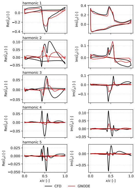
- Moving shock fronts are preserved with less smearing; the strongest remaining errors localize at the shock.
- More latent dimensions reduce phase error and variance, indicating a systematic way to trade model capacity for temporal fidelity.
- Inference takes roughly 0.7 seconds per trajectory, making the trained model cheap enough for many-query tasks like optimisation.
- Frequency analysis shows GNODE acts as a low-pass filter: first harmonics are captured accurately, but higher harmonics at the shock are underestimated.
Where Pith is reading between the lines
- Because time is continuous, GNODE can be evaluated on arbitrary time grids; a natural extension would be coupling to a structural solver with adaptive time stepping, where discrete autoregressive models require interpolation.
- The latent dimensions are never probed; interpreting them might reveal physically meaningful hidden states (e.g., wake or boundary-layer memory) and enable reduced-order insights.
- The clean separation of the test frequency k=0.3 leaves open whether the advantage transfers to unseen reduced frequencies; testing on interpolation (k=0.2/0.5) and extrapolation (k=1.0) would settle this.
- The paper itself reports that training can be unstable with augmentation and that accuracy degrades near the design-space edges; this suggests the regularisation coefficient is load-bearing and should be studied further.
Editorial analysis
A structured set of objections, weighed in public.
Referee Report
Summary. The paper proposes GNODE, a graph neural ODE with augmented latent dimensions and exogenous controls, as a continuous-time surrogate for unsteady transonic airfoil surface quantities. It is compared with an autoregressive graph-network simulator (GNS) baseline on a URANS dataset of a pitching RAE 2822 airfoil. The evaluation is internally careful: 160 HPO trials per architecture, five independent training runs, noise-perturbed teacher forcing for GNS, and metrics on both surface fields and integrated coefficients. The reported results show GNODE outperforming GNS on all metrics, with lower variance, less shock smearing, and smaller phase lag; an ablation study attributes part of this improvement to augmented latent dimensions. The authors conclude that continuous-time integration and augmentation yield a generally applicable surrogate for nonlinear spatio-temporal systems with exogenous inputs.
Significance. If the results are taken at face value, the paper makes a useful methodological contribution: GNODE directly predicts distributed surface quantities in continuous time, handles exogenous controls, and appears more stable than a discrete-time autoregressive baseline. The careful HPO, multi-seed statistics, frequency-domain analysis, and augmentation ablation are genuine strengths. However, the comparison is presently confounded by a training-objective difference, and the empirical support rests on a narrow test set. The central claim that continuous-time integration (or augmentation) is responsible for the stability gain is therefore not yet cleanly established; the paper would be substantially strengthened by an unrolled-training GNS baseline and by testing on additional reduced frequencies or near-stall conditions.
major comments (2)
- [§3.1 vs §3.3, Algorithms 1–2, Eqs. (10) and (19)] The headline comparison is confounded by the training objective. GNS is trained with one-step teacher forcing (Algorithm 1, Eq. (10)), while GNODE is trained by backpropagating through ODESolve over the full trajectory (Algorithm 2, Eq. (19)). The paper itself notes that 'unrolled training would be an alternative option that supposedly leads to improved rollout stability' (§3.1). Consequently, the large stability gap in Table 4 and Figure 8 may be due to the loss used for training, not to continuous-time integration. The authors should retrain the GNS with truncated or full trajectory loss, or train a GNODE variant with single-step loss, to isolate the architectural effect. Without such an experiment, the abstract and conclusions should be revised to compare full-trajectory training against teacher forcing rather than continuous-time against discrete-time architectures.
- [§4, test-set selection; conclusion] The generalization claim is not supported by the test distribution. All test trajectories are at a single reduced frequency k=0.3 (8 samples), and the most nonlinear cases — α0=4.5°, amplitude 0.1° — were deliberately excluded from the dataset (§4). The claim that GNODE is 'suitable to model non-linear spatio-temporal systems with exogenous inputs' therefore overreaches. Additional evaluation on at least one held-out reduced frequency (e.g., k=0.5 or k=1.0) or on near-stall conditions is needed to substantiate the general claim. If such experiments are not feasible, the conclusions should be explicitly scoped to the tested parameter regime.
minor comments (5)
- [Abstract] Typo: 'a simulations' should be 'simulations'.
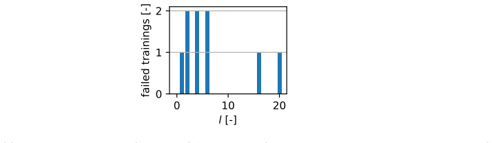
- [§5.3, Figure 11] The caption says 'failed trainings' but does not describe the retraining policy for failed runs. Clarify whether the reported means and standard deviations in Figure 12 exclude or include re-run attempts.
- [Table 2] The row 'augmentedDimension' applies only to GNODE. Marking it '—' for GNS would avoid confusion.
- [§5.3, phase-lag explanation] The explanation that hysteresis causes trajectory crossing in the unaugmented state, and that augmentation resolves it, is plausible but not demonstrated. The empirical trend in Figure 12 is the main evidence; the theoretical mechanism should be labeled a hypothesis or supported by a state-space analysis.
- [Algorithm 2] The 'context' argument is used in the pseudocode but never defined in the listing. Add a short note that it contains the motion parameters α0, α-hat, and k.
Circularity Check
No significant circularity: the empirical GNODE-vs-GNS evaluation uses held-out test data, hyperparameters are tuned on validation, and the load-bearing theoretical support (trajectory-crossing/uniqueness) is an external citation, not author self-citation.
full rationale
The paper's central claim is empirical: GNODE models are trained on 32 URANS trajectories and evaluated on 8 held-out test trajectories (Section 4), with metrics defined independently in Appendix A.2. Hyperparameters are selected by HPO on validation data (Section 5.1, Table 2) and then fixed; no fitted quantity is renamed as a prediction. The phase-lag/expressivity explanation for augmentation invokes the external trajectory-crossing/uniqueness theorem of Dupont et al. [21], not the authors' own prior work; the augmentation ablation (Section 5.3) varies l and measures phase differences on the test set, so the reported improvement is not built into the loss or the hyperparameters by construction. Self-citations [5,6,29,30] support the SMARTy implementation and prior steady-state GNN results, but they are not load-bearing for the new claims. Two concerns in the provided material are correctness/validity issues rather than circularity: (i) GNS is trained with one-step teacher forcing while GNODE is trained by backpropagating through the full ODE trajectory (Algorithm 1 vs Algorithm 2), so the stability gap may partly be a training-objective confound; the paper itself notes that unrolled training 'would be an alternative option that supposedly leads to improved rollout stability' (Section 3.1). (ii) The test set is narrow (single k=0.3; alpha0=4.5 degrees and amplitude 0.1 degrees removed, Section 4), limiting external validity. Neither issue makes the derivation equivalent to its inputs, so the circularity score is 0.
Axiom & Free-Parameter Ledger
free parameters (5)
- augmentedDimension =
14
- latentDimension (GNODE) =
186
- numberNeurons (GNODE) =
86
- regularisationFactor =
2.23e-6
- noiseLevel (GNS) =
0.0183
axioms (4)
- domain assumption URANS with negative Spalart-Allmaras turbulence model (DLR-TAU) provides an accurate reference for unsteady transonic aerodynamics of the RAE 2822 airfoil.
- standard math The uniqueness theorem for ODE initial-value problems implies unaugmented Neural ODEs cannot represent crossing trajectories, and augmentation resolves this.
- domain assumption The four training reduced frequencies (0.1, 0.2, 0.5, 1.0) and the excluded extreme cases bracket a test regime representative of dynamic linear and nonlinear transonic behavior.
- domain assumption Analytic control function f_u(t) exactly represents the pitching motion during training and inference.
Cite this review
Pith. "Pith review of Spatio-Temporal Prediction of Unsteady Airfoil Aerodynamics Using Augmented Graph Neural Ordinary Differential Equations with Exogenous Controls." pith.science (2026). https://pith.science/paper/IKN4YUU6
@misc{pith2026260718309,
  author       = {Pith},
  title        = {Pith review of: Spatio-Temporal Prediction of Unsteady Airfoil Aerodynamics Using Augmented Graph Neural Ordinary Differential Equations with Exogenous Controls},
  year         = {2026},
  howpublished = {\url{https://pith.science/paper/IKN4YUU6}},
  note         = {Machine review of arXiv:2607.18309}
}
read the original abstract
Unsteady aerodynamic phenomena, such as gusts, turbulence, and fluid-structure interactions affect an aircraft during flight. For design, optimisation and certification, it is indispensable to quantify such unsteady aerodynamic effects. Industry-standard computational fluid dynamics methods, such as solving the unsteady Reynolds-averaged Navier-Stokes equations or the linearized frequency domain method, are either computationally expensive or restricted by assumptions like linearity. Once trained, machine learning methods are capable of computing non-linear relationships very fast, making them suitable as surrogate models. By autoregressively applying graph neural networks (GNNs), operating on a discretised spatial domain, spatio-temporal predictions can be made. However, autoregressive GNNs suffer from error accumulation leading to unstable rollouts over time. Here we show that combining GNNs with augmented Neural Ordinary Differential Equations yields temporally stable predictions of the surface forces on a pitching airfoil. We found that our approach, called GNODE, based on Graph Neural Ordinary Differential Equations, provides temporally more stable, spatially smoother, and overall more accurate results than an autoregressive GNN baseline. Tests are conducted on a dataset consisting of a simulations of a pitching airfoil, including transonic shocks, transient behaviour and dynamic non-linearities. Augmenting GNODEs with additional latent dimensions improves the expressivity and accuracy by capturing underlying history effects. The developed method demonstrates an approach that is suitable to model non-linear spatio-temporal systems with exogenous inputs.
Figures




Reference graph
Works this paper leans on
-
[1]
A. F. Agarap, Deep learning using rectified linear units (relu), arXiv preprint arXiv:1803.08375 (2018)
Pith/arXiv arXiv 2018
-
[2]
Akiba, S
T. Akiba, S. Sano, T. Yanase, T. Ohta, M. Koyama, Optuna: A next-generation hyperparameter optimization framework, in: Proceedings of the 25th ACM SIGKDD international conference on knowledge discovery & data mining, 2019, pp. 2623–2631
2019
-
[3]
S. R. Allmaras, F. T. Johnson, Modifications and clarifications for the implementation of the spalart-allmaras turbulence model, in: Seventh international conference on computational fluid dynamics (ICCFD7), volume 1902, Big Island, HI, 2012, pp. 1–11
1902
-
[4]
P.W.Battaglia,J.B.Hamrick,V.Bapst,A.Sanchez-Gonzalez,V.Zambaldi,M.Malinowski,A.Tacchetti,D.Raposo,A.Santoro,R.Faulkner, et al., Relational inductive biases, deep learning, and graph networks, arXiv preprint arXiv:1806.01261 (2018)
Pith/arXiv arXiv 2018
-
[5]
Bekemeyer, A
P. Bekemeyer, A. Bertram, D. A. Hines Chaves, M. Dias Ribeiro, A. Garbo, A. Kiener, C. Sabater, M. Stradtner, S. Wassing, M. Widhalm, et al., Data-driven aerodynamic modeling using the dlr smarty toolbox, in: AIAA Aviation 2022 Forum, 2022, p. 3899
2022
-
[6]
P.Bekemeyer,A.Barklage,D.A.HinesChaves,M.Stradtner,S.Görtz, Recentadvancesindata-drivenmodelingforaerodynamicapplications using dlr’s smarty toolbox, in: AIAA SCITECH 2024 Forum, 2024, p. 0010
2024
-
[7]
Bhatnagar, Y
S. Bhatnagar, Y. Afshar, S. Pan, K. Duraisamy, S. Kaushik, Prediction of aerodynamic flow fields using convolutional neural networks, Computational Mechanics 64 (2019) 525–545
2019
-
[8]
M. M. Bronstein, J. Bruna, Y. LeCun, A. Szlam, P. Vandergheynst, Geometric deep learning: going beyond euclidean data, IEEE Signal Processing Magazine 34 (2017) 18–42
2017
-
[9]
S. L. Brunton, S. T. Dawson, C. W. Rowley, State-space model identification and feedback control of unsteady aerodynamic forces, Journal of Fluids and Structures 50 (2014) 253–270
2014
-
[10]
S. L. Brunton, J. L. Proctor, J. N. Kutz, Discovering governing equations from data by sparse identification of nonlinear dynamical systems, Proceedings of the national academy of sciences 113 (2016) 3932–3937
2016
-
[11]
S. L. Brunton, B. R. Noack, P. Koumoutsakos, Machine learning for fluid mechanics, Annual review of fluid mechanics 52 (2020) 477–508
2020
-
[12]
Bui-Thanh, M
T. Bui-Thanh, M. Damodaran, K. Willcox, Proper orthogonal decomposition extensions for parametric applications in compressible aerodynamics, in: 21st AIAA applied aerodynamics conference, 2003, p. 4213
2003
-
[13]
Y. Cao, M. Chai, M. Li, C. Jiang, Efficient learning of mesh-based physical simulation with bi-stride multi-scale graph neural network, in: International conference on machine learning, PMLR, 2023, pp. 3541–3558
2023
-
[14]
Catalani, S
G. Catalani, S. Agarwal, X. Bertrand, F. Tost, M. Bauerheim, J. Morlier, Neural fields for rapid aircraft aerodynamics simulations, Scientific Reports 14 (2024) 25496
2024
-
[15]
Chen,Y.Rubanova,J
R.T. Chen,Y.Rubanova,J. Bettencourt,D.K.Duvenaud, Neuralordinary differentialequations, Advances inneuralinformationprocessing systems 31 (2018)
2018
-
[16]
R. T. Q. Chen, torchdiffeq, 2018. URL:https://github.com/rtqichen/torchdiffeq
2018
-
[17]
K. Cho, B. Van Merriënboer, Ç. Gulçehre, D. Bahdanau, F. Bougares, H. Schwenk, Y. Bengio, Learning phrase representations using rnn encoder–decoder for statistical machine translation, in: Proceedings of the 2014 conference on empirical methods in natural language processing (EMNLP), 2014, pp. 1724–1734
2014
-
[18]
Colombo, M
M. Colombo, M. Bauerheim, J. Morlier, Data driven prediction of gust aeroelastic dynamics of hale using graph neural ordinary differential equations with input control, Aerospace Science and Technology (2025) 111505
2025
-
[19]
P. Cook, M. Firmin, M. McDonald, Aerofoil RAE 2822: pressure distributions, and boundary layer and wake measurements, RAE, 1977
1977
-
[20]
C. F. Curtiss, J. O. Hirschfelder, Integration of stiff equations, Proceedings of the national academy of sciences 38 (1952) 235–243
1952
-
[21]
Dupont, A
E. Dupont, A. Doucet, Y. W. Teh, Augmented neural odes, Advances in neural information processing systems 32 (2019)
2019
-
[22]
EASA, Certification specifications and acceptable means of compliance for large aeroplanes, 2023
2023
-
[23]
M. Fey, J. E. Lenssen, Fast graph representation learning with pytorch geometric, arXiv preprint arXiv:1903.02428 (2019)
Pith/arXiv arXiv 1903
-
[24]
Friedewald, Gust-Induced Amplitude Effects in Transonic Flow, Ph.D
D. Friedewald, Gust-Induced Amplitude Effects in Transonic Flow, Ph.D. thesis, Technische Universität Braunschweig, 2025
2025
-
[25]
Fronk, L
C. Fronk, L. Petzold, Training stiff neural ordinary differential equations with implicit single-step methods, Chaos: An Interdisciplinary Journal of Nonlinear Science 34 (2024)
2024
-
[26]
T. Gao, S. Sun, H. Liu, H. Gao, Global convergence in neural odes: Impact of activation functions, arXiv preprint arXiv:2509.22436 (2025)
arXiv 2025
-
[27]
X. Han, H. Gao, T. Pfaff, J.-X. Wang, L.-P. Liu, Predicting physics in mesh-reduced space with temporal attention, arXiv preprint arXiv:2201.09113 (2022)
Pith/arXiv arXiv 2022
-
[28]
L. Harsch, S. Riedelbauch, Direct prediction of steady-state flow fields in meshed domain with graph networks, arXiv preprint arXiv:2105.02575 (2021)
Pith/arXiv arXiv 2021
-
[29]
D.Hines,P.Bekemeyer, Graphneuralnetworksforthepredictionofaircraftsurfacepressuredistributions, AerospaceScienceandTechnology 137 (2023) 108268
2023
-
[30]
Hines, P
D. Hines, P. Bekemeyer, Prediction of surface pressure distributions of non-parametric airfoils using geometric deep learning methods, Computers & Fluids (2026) 106979
2026
-
[31]
Hochreiter, Long short-term memory, Neural Computation MIT-Press (1997)
S. Hochreiter, Long short-term memory, Neural Computation MIT-Press (1997)
1997
-
[32]
Hornik, M
K. Hornik, M. Stinchcombe, H. White, Multilayer feedforward networks are universal approximators, Neural networks 2 (1989) 359–366
1989
-
[33]
Jameson, Application of dual time stepping to fully implicit runge kutta schemes for unsteady flow calculations, in: 22nd AIAA Computational Fluid Dynamics Conference, 2015, p
A. Jameson, Application of dual time stepping to fully implicit runge kutta schemes for unsteady flow calculations, in: 22nd AIAA Computational Fluid Dynamics Conference, 2015, p. 2753
2015
-
[34]
D. P. Kingma, J. Ba, Adam: A method for stochastic optimization, arXiv preprint arXiv:1412.6980 (2014)
Pith/arXiv arXiv 2014
-
[35]
G.Kohl,L.-W.Chen,N.Thuerey, Benchmarkingautoregressiveconditionaldiffusionmodelsforturbulentflowsimulation, NeuralNetworks (2026) 108641
2026
-
[36]
J. N. Kutz, S. L. Brunton, B. W. Brunton, J. L. Proctor, Dynamic mode decomposition: data-driven modeling of complex systems, SIAM, 2016
2016
-
[37]
:Preprint submitted to Elsevier Page 26 of 27
A.M.Lamb,A.G.ALIASPARTHGOYAL,Y.Zhang,S.Zhang,A.C.Courville,Y.Bengio, Professorforcing:Anewalgorithmfortraining recurrent networks, Advances in neural information processing systems 29 (2016). :Preprint submitted to Elsevier Page 26 of 27
2016
-
[38]
Langer, An initial investigation of solving rans equations in combination with two-equation turbulence models, 2019
S. Langer, An initial investigation of solving rans equations in combination with two-equation turbulence models, 2019
2019
-
[39]
LeCun, Y
Y. LeCun, Y. Bengio, G. Hinton, Deep learning, nature 521 (2015) 436–444
2015
-
[40]
Massegur, A
D. Massegur, A. Da Ronch, Recurrent graph convolutional multi-mesh autoencoder for unsteady transonic aerodynamics, Journal of Fluids and Structures 131 (2024) 104202
2024
-
[41]
Øksendal, Stochastic differential equations, in: Stochastic differential equations: an introduction with applications, Springer, 2003, pp
B. Øksendal, Stochastic differential equations, in: Stochastic differential equations: an introduction with applications, Springer, 2003, pp. 38–50
2003
-
[42]
Y. Pan, X. An, Y. Lei, C. Ji, An improved neural network for modeling airfoil’s unsteady aerodynamics in transonic flow, Physics of Fluids 36 (2024)
2024
-
[43]
Paszke, S
A. Paszke, S. Gross, F. Massa, A. Lerer, J. Bradbury, G. Chanan, T. Killeen, Z. Lin, N. Gimelshein, L. Antiga, et al., Pytorch: An imperative style, high-performance deep learning library, Advances in neural information processing systems 32 (2019)
2019
-
[44]
T. Pfaff, M. Fortunato, A. Sanchez-Gonzalez, P. W. Battaglia, Learning mesh-based simulation with graph networks, arXiv preprint arXiv:2010.03409 (2020)
Pith/arXiv arXiv 2010
-
[45]
M.Poli,S.Massaroli,J.Park,A.Yamashita,H.Asama,J.Park, Graphneuralordinarydifferentialequations, arXivpreprintarXiv:1911.07532 (2019)
Pith/arXiv arXiv 1911
-
[46]
Pontryagin, Mathematical Theory of Optimal Processes, Classics of Soviet Mathematics, Taylor & Francis, 1987
L. Pontryagin, Mathematical Theory of Optimal Processes, Classics of Soviet Mathematics, Taylor & Francis, 1987
1987
-
[47]
M. D. Ribeiro, M. Stradtner, P. Bekemeyer, Unsteady reduced order model with neural networks and flight-physics-based regularization for aerodynamic applications, Computers & Fluids 264 (2023) 105949
2023
-
[48]
Sanchez-Gonzalez, J
A. Sanchez-Gonzalez, J. Godwin, T. Pfaff, R. Ying, J. Leskovec, P. Battaglia, Learning to simulate complex physics with graph networks, in: International conference on machine learning, PMLR, 2020, pp. 8459–8468
2020
-
[49]
Sabater, P
C. Sabater, P. Stürmer, P. Bekemeyer, Fast predictions of aircraft aerodynamics using deep-learning techniques, Aiaa Journal 60 (2022) 5249–5261
2022
-
[50]
P. J. Schmid, Dynamic mode decomposition of numerical and experimental data, Journal of fluid mechanics 656 (2010) 5–28
2010
-
[51]
M.Schroeder,Synthesisoflow-peak-factorsignalsandbinarysequenceswithlowautocorrelation(corresp.),IEEEtransactionsonInformation Theory 16 (1970) 85–89
1970
-
[52]
Schwamborn, A
D. Schwamborn, A. Gardner, H. von Geyr, A. Krumbein, H. Lüdeke, A. Stürmer, Development of the tau-code for aerospace applications, 2008
2008
-
[53]
Serrano, L
L. Serrano, L. Le Boudec, A. Kassaï Koupaï, T. X. Wang, Y. Yin, J.-N. Vittaut, P. Gallinari, Operator learning with neural fields: Tackling pdes on general geometries, Advances in Neural Information Processing Systems 36 (2023) 70581–70611
2023
-
[54]
L. Serrano, L. Migus, Y. Yin, J. A. Mazari, P. Gallinari, Infinity: Neural field modeling for reynolds-averaged navier-stokes equations, arXiv preprint arXiv:2307.13538 (2023)
Pith/arXiv arXiv 2023
-
[55]
W. A. Silva, Application of nonlinear systems theory to transonic unsteady aerodynamic responses, Journal of aircraft 30 (1993) 660–668
1993
-
[56]
I. M. Sobol, Y. L. Levitan, On the use of variance reducing multipliers in monte carlo computations of a global sensitivity index, Computer Physics Communications 117 (1999) 52–61
1999
-
[57]
Stickan, Explanation of aerostabil limit-cycle oscillations via high-fidelity aeroelastic simulations, 2018
B. Stickan, Explanation of aerostabil limit-cycle oscillations via high-fidelity aeroelastic simulations, 2018
2018
-
[58]
Tang, Orthogonal array-based latin hypercubes, Journal of the American statistical association 88 (1993) 1392–1397
B. Tang, Orthogonal array-based latin hypercubes, Journal of the American statistical association 88 (1993) 1392–1397
1993
-
[59]
Thormann, M
R. Thormann, M. Widhalm, Linear-frequency-domain predictions of dynamic-response data for viscous transonic flows, AIAA journal 51 (2013) 2540–2557
2013
-
[60]
Vaswani, N
A. Vaswani, N. Shazeer, N. Parmar, J. Uszkoreit, L. Jones, A. N. Gomez, Ł. Kaiser, I. Polosukhin, Attention is all you need, Advances in neural information processing systems 30 (2017)
2017
-
[61]
Weiss, A tutorial on the proper orthogonal decomposition, in: AIAA aviation 2019 forum, 2019, p
J. Weiss, A tutorial on the proper orthogonal decomposition, in: AIAA aviation 2019 forum, 2019, p. 3333
2019
-
[62]
Y. Yang, K. Pahlke, Implementation of a dual-time stepping method for the numerical solution of ns equations for rigid airfoils in arbitrary unsteady motion, 1995
1995
-
[63]
R. Zahn, M. Winter, M. Zieher, C. Breitsamter, Application of a long short-term memory neural network for modeling transonic buffet aerodynamics, Aerospace Science and Technology 113 (2021) 106652. :Preprint submitted to Elsevier Page 27 of 27
2021
This paper was first reviewed by deepseek-v4-flash on August 1, 2026.
discussion (0)
Sign in with ORCID, Apple, or X to comment. Anyone can read and Pith papers without signing in.