REVIEW 2 major objections 4 minor 76 references
Bivariate Archimax copulas become identifiable when viewed through a one-parameter transformation of their generator and Pickands dependence function.
Reviewed by Pith at T0; open to challenge. T0 means a machine referee read the full paper against a public rubric. the ladder, T0–T4 →
T0 review · deepseek-v4-flash
2026-08-01 13:29 UTC pith:I6NSW5YE
load-bearing objection New identifiability result is real; the consistency claim needs a caveat — but worth refereeing. the 2 major comments →
Identifiability, Convergence and Nonparametric Estimation of Bivariate Archimax Copulas
The pith
A machine-rendered reading of the paper's core claim, the machinery that carries it, and where it could break.
Core claim
The central claim is that the pair (ψ)^{1−τ_A} and (A)^{1−τ_A} identifies the Archimax copula C_{ψ,A} uniquely, where τ_A is Kendall's τ of the extreme-value copula induced by A. This resolves the non-identifiability that blocked fully nonparametric estimation. The same transformed functions govern convergence: uniform convergence of Archimax copulas is equivalent to uniform convergence of (ψ_n)^{1−τ_{A_n}} and (A_n)^{1−τ_{A_n}}, and also to weak conditional convergence of the copulas' Markov kernels. The paper exploits these equivalences to build estimators C^Ξ_{α_n,n} that are elements of the Archimax family and satisfy d_∞(C^Ξ_{α_n,n}, C_{ψ,A}) → 0 almost surely under stated regularity co
What carries the argument
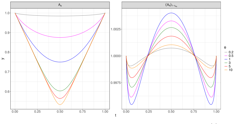
The engine is the transformation (ψ)^α(z) = ψ(z^α) and (A)^α(t) = (t^α+(1−t)^α)^{1/α} A^{1/α}(t^α/(t^α+(1−t)^α)), applied with α = 1−τ_A. The key identity is that the Kendall distribution function of any Archimax copula C_{ψ,A} equals the Kendall distribution function of the Archimedean copula with generator (ψ)^{1−τ_A}; this links the whole estimation problem to the empirically accessible Kendall distribution. Estimation proceeds by estimating (ψ)^{1−τ_A} from the empirical Kendall distribution, estimating (A)^{1−τ_A} by Pickands-type or CFG-type formulas, projecting the result onto the set of Pickands functions via the greatest convex minorant, and choosing an exponent α_n by an optimizati
Load-bearing premise
The consistency theorems rest on moment conditions—E[Z] < ∞ for the Pickands estimator and E[|log Z|] < ∞ for the CFG estimator—plus tail-integral bounds (Assumptions 1–3) that can fail for perfectly separated ranks, and the paper itself shows E[Z] = ∞ for Clayton generators whenever θ ≥ 1−τ_A.
What would settle it
Simulate Clayton-based Archimax data with θ ≥ 1−τ_A and check whether the Pickands estimator's uniform distance to the truth fails to converge to zero as n grows; separately, take the perfectly separated rank configuration W_i = (i−1)/(n+1), where the paper's Remark 9 shows Assumption 2 is violated, and test whether the CFG estimator's consistency proof breaks down in finite samples.
If this is right
- A fully nonparametric, strongly consistent estimator that stays inside the Archimax family now exists for bivariate copulas.
- Uniform convergence in the Archimax family is equivalent to weak conditional convergence, so dependence measures continuous under that convergence—including Chatterjee's ξ and Trutschnig's ζ₁—can be estimated by plugging the fitted copula in directly.
- Two different generator/Pickands pairs can represent the same Archimax copula only when linked through the exponent 1−τ_A; fixing τ_A makes the original pair identifiable.
- The CFG-type estimator is reported to outperform both the empirical copula estimator and the Pickands-type estimator in the simulations, with especially large gains near the Clayton boundary where the Pickands estimator's moment condition fails.
- On real precipitation maxima from Bregenz and Dornbirn, the CFG Archimax estimator lies closer to the empirical copula than a nonparametric extreme-value CFG estimator, suggesting a better fit when lower-tail dependence is present.
Where Pith is reading between the lines
- The identifiability trick—scaling ψ and A by the same power 1−τ_A—is a natural template for multivariate Archimax models, where non-identifiability is even more severe; the paper does not make that extension, but the ratio-symmetric form of the transformation suggests it.
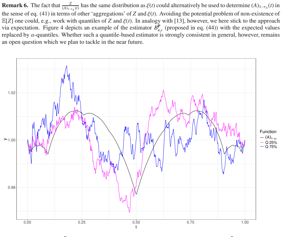
- The paper's Remark 6 sketches a quantile-based analogue of the Pickands estimator that would avoid the restrictive E[Z] < ∞ condition entirely; proving its strong consistency is a concrete open problem that would extend the method to heavy-tailed generators like Clayton beyond θ = 1−τ_A.
- Section 7's real-data conclusions rely on an unproved extension of the i.i.d. theorems to stationary α-mixing sequences; if that extension is valid, the estimator becomes applicable to the time-series settings that originally motivated extreme-value copula modeling in hydrology and finance.
- The empirical-Kendall step suggests the same machinery could estimate the transformed generator for any copula with a known Kendall distribution, giving a route to semiparametric Archimax models in higher dimensions even before full multivariate identifiability is settled.
Editorial analysis
A structured set of objections, weighed in public.
Referee Report
Summary. The paper studies bivariate Archimax copulas, the class C_am that contains both Archimedean and extreme-value copulas. Its main theoretical contributions are (i) an identifiability result (Theorem 2): two Archimax copulas coincide iff their transformed generators (ψ)^{1−τ_A} and transformed Pickands functions (A)^{1−τ_A} coincide; (ii) a convergence theorem (Theorem 3) showing that uniform convergence, uniform convergence of the transformed components, and weak conditional convergence are equivalent in C_am \ {M}; and (iii) two nonparametric estimators, a Pickands-type and a CFG-type estimator, both of which produce copulas inside C_am, together with strong consistency claims (Theorems 4–6) and plug-in consistency for dependence measures such as Chatterjee's ξ and Trutschnig's ζ1. The paper also contains a large simulation study and a real-data application to precipitation records.
Significance. If the consistency theorem were fully established, the paper would resolve a genuine gap: no fully nonparametric, family-preserving estimator for Archimax copulas was previously available. The identifiability result and the convergence equivalence are substantial and appear to be correct; the ratio identities underlying the estimator (eqs. 40–42) check out by direct computation. The paper is also unusually transparent about open questions and limitations, including the quantile-based alternative in Remark 6 and the failure of moment conditions for Clayton generators in Lemma 29. The simulation study is extensive and the real-data example is a useful illustration. However, the advertised strong consistency is not actually proved as stated, because the proofs rely on sample-dependent regularity assumptions whose a.s. validity is not established.
major comments (2)
- [Appendix B.5 / Theorem 4] Assumptions 1–3 are conditions on the sample-dependent estimator φ_n, not on the true pair (ψ, A). Lemma 16 and Lemma 18 use them to obtain the moment convergence required for Theorem 4, but the paper does not prove that these assumptions hold almost surely along the sample path, nor that their failure occurs only finitely often. Remark 9 explicitly gives a finite-sample configuration (perfectly separated ranks) on which Assumption 2 fails, and no argument excludes infinitely many such failures with positive probability. Consequently, the a.s. strong consistency of the CFG estimator, as claimed in the abstract and Theorem 4, is not established for the models stated.
- [Lemma 29 / Section 6.1 / Figure 6] For the Pickands variant, the moment condition E[Z]<∞ fails for the Clayton family whenever θ ≥ 1−τ_A. Since Clayton copulas are a standard subfamily of Archimax copulas, the abstract's unqualified claim that both estimators are 'strongly consistent under mild regularity conditions' is misleading for the Pickands estimator; either the statement must be explicitly restricted or the abstract should not present both estimators as having the same guarantee. The simulation results (Figure 6 and Tables C.18–C.20) confirm the practical deterioration, so this is not a purely technical caveat.
minor comments (4)
- [Theorem 4 statement] The sample is written '(X1, X1), (X2, Y2),...' but should be '(X1, Y1), (X2, Y2),...'.
- [Section 6.1] The text says 'As shown in Lemma 1, E[log Z] exists for all families considered' but the correct reference is Lemma 29 in Appendix B.5, not Lemma 1 (which concerns h_A).
- [Section 7] The real-data section states 'we conjecture that our results extend to stationary α-mixing sequences' and then proceeds to apply the estimator and interpret the results. The attached tests (ADF, Ljung–Box, Box–Pierce) do not establish α-mixing; they only fail to reject certain independence/stationarity hypotheses. The practical conclusions should be explicitly framed as heuristic, conditional on an unproved extension.
- [Appendix B.5, Remark 9] The displayed calculation of ∫_0^{1/2} s/(K_n(s)−s) dλ(s) ≥ n/2 is correct, but the sentence following it contains a small grammatical issue ('this shows that in this situation Assumption 2 does not hold' could be clearer as 'Assumption 2 fails for this configuration').
Circularity Check
No load-bearing circularity: identifiability and estimator consistency are derived in-paper from the Archimax representation and published external/rival results; self-citations are dense but not used to smuggle in the conclusions.
full rationale
The central identifiability theorem (Theorem 2) is proved using Lemma 6, which follows by direct computation from the Kendall distribution formula (22) and the Archimedean characterization (13); the conclusion that transformed generators and transformed Pickands functions identify the copula is not assumed as an input. The convergence theorem (Theorem 3) is established through the paper's own Lemmas 8–12, with the Archimedean part relying on the published, peer-reviewed [39] rather than on an unverified self-citation. The estimator claims (Theorems 4–6) are based on the representations (41)–(42), which are derived from the survival identity P[ξ(t)>x]=(ψ)^{1−τ_A}(x (A)^{1−τ_A}(t)), and the consistency proof is a standard plug-in/empirical-risk argument comparing the selected α_n to the population value τ_A (Lemma 27 and the proof of Theorem 4). No fitted parameter is renamed as a prediction, and no quantity is defined in terms of the quantity it is supposed to establish. The paper does contain explicit limitations that are not circularity: Assumptions 1–3 are sample-path tail conditions that are not proved to hold almost surely (Remark 9 shows Assumption 2 can fail), Lemma 29 excludes Clayton generators with θ≥1−τ_A for the Pickands variant, and Section 7 states that the α-mixing extension is only a conjecture. These are correctness/robustness concerns, not circular reductions. Self-citation is frequent (e.g., Lemmas 6, Theorem 1, eq. (22), [38,39]), and [39] shares the second author, but those results are published, parameter-free, and do not assume the target Archimax conclusions, so they count as external evidence under the review rules. Overall, the derivation chain is self-contained against the Archimax formula and established Archimedean/EV theory; the only score contribution is the density of self-citations, which is not load-bearing.
Axiom & Free-Parameter Ledger
free parameters (2)
- α_n — optimization index =
argmin over [0, 1−1/n] of ||C^Ξ_{α,n} − D^Ξ_n||_∞ (eq 49); reported α_n ≈ 0.4368 on the rainfall data
- ε_n — positivity correction =
exp(−n)
axioms (5)
- domain assumption F^K_{ψ,A}(t) = τ_A t + (1−τ_A) F^K_ψ(t) (eq 22)
- domain assumption Markov kernel representation of C_{ψ,A} (Theorem 1, from [17, Thm 4.1])
- standard math In C_ar and C_ev uniform convergence ⟺ generator/Pickands convergence ⟺ weak conditional convergence ([39])
- domain assumption Moment conditions: E[Z] < ∞ (Pickands) or E[|log Z|] < ∞ (CFG), plus Assumptions 1–3
- standard math Kendall's τ integration formulas (eqs 8, 9, 19)
read the original abstract
Considering that the family of bivariate Archimax copulas contains both the Archimedean and the extreme-value class, Archimax copulas constitute a flexible family allowing to model extreme and moderate levels of dependence. Despite their appeal, no fully nonparametric, consistent estimator that is itself an element of the Archimax family $\mathcal{C}_{am}$ has been established yet, mainly because Archimedean generators and Pickands dependence functions alone do not identify Archimax copulas. We resolve this identifiability issue by working with transformed generators and transformed Pickands dependence functions, and show that these functions do identify the Archimax copula uniquely. Building upon this result, we prove that uniform convergence of Archimax copulas is equivalent to uniform convergence of the corresponding transformed generators and Pickands dependence functions. Moreover, as for Archimedean and extreme-value copulas, uniform convergence in $\mathcal{C}_{am}$ is equivalent to weak convergence of almost all conditional distributions. Exploiting these equivalences, we construct two nonparametric estimators for Archimax copulas (a Pickands and a CFG type estimator, both elements of $\mathcal{C}_{am}$) and show that they are strongly consistent under mild regularity conditions. As a further consequence of the aforementioned weak conditional convergence, we obtain strongly consistent plug-in estimators for measures of directed dependence such as Chatterjee's $\xi$ and Trutschnig's $\zeta_1$. A large-scale simulation study shows that the proposed CFG type estimator outperforms both the standard empirical copula estimator and the Pickands type estimator; an application to precipitation data from Bregenz and Dornbirn (Austria) illustrates the practical use of our estimators on real data.
Figures






Reference graph
Works this paper leans on
-
[1]
Ansari, P .B
J. Ansari, P .B. Langthaler, S. Fuchs and W . Trutschnig: Q uantifying and estimating dependence via sensitivity of conditional distributions, Bernoulli 32 (2026), 179–204
2026
-
[2]
T. Bacigál: acopula: Modelling dependence with multiva riate Archimax (or any user-defined continuous) copu- las, R package version 0.9.4, https://CRAN.R-project.org/package=acopula (2023)
2023
-
[3]
Bacigál, V
T. Bacigál, V . Jágr, J. Segers and R. Mesiar: Non-exchang eable random variables, Archimax copulas and their fitting to real data, Kybernetika 4 (2011), 519–531
2011
-
[4]
Barbe, C
P . Barbe, C. Genest, K. Ghoudi and B. Rémillard: On Kendal l’s process, J. Multivar . Anal.58 (1996), 197–229
1996
-
[5]
Beirlant, Y
J. Beirlant, Y . Goegebeur, J. Segers and J. Teugels: Stat istics of extremes: Theory and applications, Wiley Series in Probability and Statistics, John Wiley and Sons Ltd., Chi chester (2004)
2004
-
[6]
Box and D.A
G.E.P . Box and D.A. Pierce: Distribution of residual cor relations in autoregressive-integrated moving average time series models, J. Am. Stat. Assoc. 65 (1970), 1509–1526
1970
-
[7]
Bücher, H
A. Bücher, H. Dette and S. V olgushev: New estimators of th e Pickands dependence function and a test for extreme-value dependence, Ann. Stat. 39 (2011), 1963–2006
2011
-
[8]
Capéraà and A.-L
P . Capéraà and A.-L. Fougères: Estimation of a bivariate extreme value distribution, Extremes 3 (2000), 311– 329
2000
-
[9]
Capéraà, A.-L
P . Capéraà, A.-L. Fougères and C. Genest: A nonparametri c estimation procedure for bivariate extreme value copulas, Biometrika 84 (1997), 567–577
1997
-
[10]
Capéraà, A.-L
P . Capéraà, A.-L. Fougères and C. Genest: Bivariate dis tributions with given extreme value attractor, J. Multivar . Anal. 72 (2000), 30–49
2000
-
[11]
Charpentier, A.-L
A. Charpentier, A.-L. Fougères, C. Genest and J.G. Nešl ehová: Multivariate Archimax copulas, J. Multivar . Anal. 126 (2014), 118–136
2014
-
[12]
Charpentier and J
A. Charpentier and J. Segers: Convergence of Archimede an copulas, Stat. Probab. Lett. 78 (2008), 412–419
2008
-
[13]
Chatelain, A.-L
S. Chatelain, A.-L. Fougères and J.G. Nešlehová: Infer ence for Archimax copulas, Ann. Stat. 48 (2020), 1025– 1051
2020
-
[14]
Chatelain, S
S. Chatelain, S. Perreault, A.-L. Fougères and J.G. Neš lehová: Clustered Archimax copulas, Electron. J. Stat. 19 (2025), 314–360
2025
-
[15]
Chatterjee: A new coe fficient of correlation, J
S. Chatterjee: A new coe fficient of correlation, J. Am. Stat. Assoc. 116 (2021), 2009–2022
2021
-
[16]
Cormier, C
E. Cormier, C. Genest and J.G. Nešlehová: Using B-splin es for nonparametric inference on bivariate extreme- value copulas, Extremes 17 (2014), 633–659
2014
-
[17]
N. Dietrich: On bivariate Archimax copulas: Level sets , mass distributions and related results, Extremes (2026), https://doi.org/10.1007/s10687-025-00523-6
-
[18]
Dietrich and W
N. Dietrich and W . Trutschnig: On di fferentiability and mass distributions of typical bivariate copulas, Fuzzy Sets Syst. 498 (2025), 109150
2025
-
[19]
Durante, J
F. Durante, J. Fernández Sánchez and C. Sempi: A note on b ivariate Archimax copulas, Depend. Model. 6 (2018), 178–182
2018
-
[20]
Durante and C
F. Durante and C. Sempi: Principles of copula theory, Ch apman and Hall/CRC (2015). 42
2015
-
[21]
Fernández Sánchez and W
J. Fernández Sánchez and W . Trutschnig: Singularity as pects of Archimedean copulas, J. Math. Anal. Appl. 432 (2015), 103–113
2015
-
[22]
Fils-Villetard, A
A. Fils-Villetard, A. Guillou and J. Segers: Projectio n estimators of Pickands dependence functions, Can. J. Stat. 36 (2008), 369–382
2008
-
[23]
Fuchs and M
S. Fuchs and M. Tschimpke: Total positivity of copulas f rom a Markov kernel perspective, J. Math. Anal. Appl. 518 (2023), 126629
2023
-
[24]
Fuller: Introduction to statistical time series, 2nd edition, John Wiley and Sons, New Y ork (1996)
W .A. Fuller: Introduction to statistical time series, 2nd edition, John Wiley and Sons, New Y ork (1996)
1996
-
[25]
Genest, J.G
C. Genest, J.G. Nešlehová and J. Ziegel: Inference in mu ltivariate Archimedean copula models, TEST 20 (2011), 223–256
2011
-
[26]
Genest and L.-P
C. Genest and L.-P . Rivest: Statistical inference proc edures for bivariate Archimedean copulas, J. Amer . Statist. Assoc. 88 (1993), 1034–1043
1993
-
[27]
Genest and J
C. Genest and J. Segers: Rank-based inference for bivar iate extreme-value copulas, Ann. Stat. 37 (2009), 2990–3022
2009
-
[28]
Ghorbal, C
N. Ghorbal, C. Genest and J.G. Nešlehová: On the Ghoudi, Khoudraji, and Rivest test for extreme-value dependence, Can. J. Stat. 37 (2009), 534–552
2009
-
[29]
Ghoudi, A
K. Ghoudi, A. Khoudraji and L.-P . Rivest: Propriétés st atistiques des copules de valeurs extrêmes bidimension- nelles, Can. J. Stat. 26 (1998), 187–197
1998
-
[30]
Haan and S.I
L.d. Haan and S.I. Resnick: Limit theory for multivaria te sample extremes, Probab. Theory Relat. Fields 40 (1977), 317–337
1977
-
[31]
Harvey: Time series models, 2nd edition, Harveste r Wheatsheaf, New Y ork (1993)
A.C. Harvey: Time series models, 2nd edition, Harveste r Wheatsheaf, New Y ork (1993)
1993
-
[32]
Hofert, R
M. Hofert, R. Huser and A. Prasad: Hierarchical Archima x copulas, J. Multivar . Anal.167 (2018), 195–211
2018
-
[33]
Janssen, J
P . Janssen, J. Swanepoel and N. V eraverbeke: Large samp le behavior of the Bernstein copula estimator, J. Stat. Plan. Inference 142 (2012), 1189–1197
2012
-
[34]
Joe: Dependence modeling with copulas, CRC Press (2014)
H. Joe: Dependence modeling with copulas, CRC Press (2014)
2014
-
[35]
Junker, F
R.R. Junker, F. Griessenberger and W . Trutschnig: Esti mating scale-invariant directed dependence of bivariate distributions, Comput. Stat. Data Anal. 153 (2021), 107058
2021
-
[36]
Kallenberg: Foundations of modern probability, Spr inger-V erlag, New Y ork (2002)
O. Kallenberg: Foundations of modern probability, Spr inger-V erlag, New Y ork (2002)
2002
-
[37]
Kannan and C.K
R. Kannan and C.K. Krueger: Advanced analysis on the rea l line, Springer V erlag, New Y ork (1996)
1996
-
[38]
Kasper, N
T. Kasper, N. Dietrich and W . Trutschnig: On convergenc e and mass distributions of multivariate Archimedean copulas and their interplay with the Williamson transform, J. Math. Anal. Appl. 529 (2024), 127555
2024
-
[39]
Kasper, S
T. Kasper, S. Fuchs and W . Trutschnig: On weak condition al convergence of bivariate Archimedean and extreme value copulas, and consequences to nonparametric estimati on, Bernoulli 27 (2021), 2217–2240
2021
-
[40]
Klenke: Wahrscheinlichkeitstheorie, Springer Leh rbuch Masterclass Series, Berlin Heidelberg (2008)
A. Klenke: Wahrscheinlichkeitstheorie, Springer Leh rbuch Masterclass Series, Berlin Heidelberg (2008)
2008
-
[41]
Kojadinovic and J
I. Kojadinovic and J. Y an: Nonparametric rank-based te sts of bivariate extreme-value dependence, J. Multivar . Anal. 101 (2010), 2234–2249
2010
-
[42]
Ljung and G.E.P
G.M. Ljung and G.E.P . Box: On a measure of lack of fit in tim e series models, Biometrika 65 (1978), 297–303
1978
-
[43]
Longin and B
F. Longin and B. Solnik: Extreme correlation of interna tional equity markets, J. Financ. 56 (2001), 649–676. 43
2001
-
[44]
Mai and M
J. Mai and M. Scherer: Bivariate extreme-value copulas with discrete Pickands dependence measure, Extremes 14 (2011), 311–324
2011
-
[45]
McNeil, R
A. McNeil, R. Frey and P . Embrechts: Quantitative risk m anagement, New Jersey, Princeton University Press (2005)
2005
-
[46]
McNeil and J
A. McNeil and J. Nešlehová: Multivariate Archimedean c opulas, d-monotone functions and ℓ1-norm symmetric distributions, Ann. Stat. 37 (2009), 3059–3097
2009
-
[47]
Mesiar and V
R. Mesiar and V . Jágr: d-Dimensional dependence functi ons and Archimax copulas, Fuzzy Sets Syst. 228 (2013), 78–87
2013
-
[48]
Nelsen: An introduction to copulas, Springer Seri es in Statistics, Springer, New Y ork, second edition (2006)
R.B. Nelsen: An introduction to copulas, Springer Seri es in Statistics, Springer, New Y ork, second edition (2006)
2006
-
[49]
Y . Ng, A. Hasan and V . Tarokh: Inference and sampling for Archimax copulas, in Advances in Neural Informa- tion Processing Systems 35 (2022), Article No. 1244, 17099– 17116
2022
-
[50]
Pickands: Multivariate extreme value distribution s, Proc
J. Pickands: Multivariate extreme value distribution s, Proc. 43rd Sess. Int. Stat. Inst. 2 (1981), 859–878
1981
-
[51]
Pollard: A user’s guide to measure theoretic probabi lity, Cambridge University Press (2001)
D. Pollard: A user’s guide to measure theoretic probabi lity, Cambridge University Press (2001)
2001
-
[52]
Salvadori, C
G. Salvadori, C. De Michele, N.T. Kottegoda and R. Rosso : Extremes in nature – an approach using copulas, Springer Dordrecht (2007)
2007
-
[53]
Schilling, R
R. Schilling, R. Song and Z. V ondracek: Bernstein funct ions: Theory and applications, De Gruyter Studies in Mathematics, De Gruyter (2012)
2012
-
[54]
Segers: Non-parametric inference for bivariate ext reme-value copulas, CentER Discussion Paper No
J. Segers: Non-parametric inference for bivariate ext reme-value copulas, CentER Discussion Paper No. 2004-91 (2004), Catholic University of Louvain (UCL)
2004
-
[55]
Trutschnig, M
W . Trutschnig, M. Schreyer and J. Fernández Sánchez: Ma ss distributions of two-dimensional extreme-value copulas and related results, Extremes 19 (2016), 405–427
2016
-
[56]
Trutschnig: On a strong metric on the space of copulas and its induced dependence measure, J
W . Trutschnig: On a strong metric on the space of copulas and its induced dependence measure, J. Math. Anal. Appl. 384 (2011), 690–705
2011
-
[57]
van der V aart: Asymptotic statistics, Cambridge S eries in Statistical and Probabilistic Mathematics
A.W . van der V aart: Asymptotic statistics, Cambridge S eries in Statistical and Probabilistic Mathematics. Cambridge University Press, Cambridge (1998). 44 Appendix A. Auxiliary lemmas and proofs In this short section, we present two auxiliary lemmas on pro perties of the generator ψ ∈ Ψ and the Pickands depen- dence function A ∈ A, which we use in Sect...
1998
-
[58]
ψn n→∞ − →(ψ)1−τA uniformly on [0, ∞)
-
[59]
ϕn(x) n→∞ − →(ϕ)1−τA(x) pointwise for every x ∈ (0, 1]
-
[60]
βn(t) n→∞ − →(β)1−τA(t) = (1 −τA)β(t) for every t ∈ I at whichβ is continuous. Proof. The first assertion has already been shown in Section 5.2, the second one is a direct consequence of the equivalences in [39, Theorem 4.1]. To prove the third statem ent recall that we have Kn(t) = t −βn(t) as well as F K ψ,A(t) = F K C(ψ)1−τA (t) = t − (β)1−τA(t). for ev...
-
[61]
There exists some constant K n ∈ (0, ∞) such that A M(t) ≤ BΞ n,c(t) ≤ Kn holds for every t ∈ I. 52
-
[62]
BΞ n,c is uniformly continuous on I
-
[63]
BΞ n,c(t)> AM(t) for every t ∈ (0, 1) and B Ξ n,c(0) = BΞ n,c(1) = 1. Proof. We start with the first assertion. For every i ∈ {1,..., n} and t ∈ I we obviously have that ϕn ( 1 n+1 ) min {1 t, 1 1−t } ≥ ˆξn,i(t) ≥ϕn ( n n+1 ) min {1 t, 1 1−t } with min {1 t, 1 1−t } = 1 for t = 0 and min {1 t, 1 1−t } = 1 for t = 1. Both, for BP n,u and for BCFG n,u it the...
-
[64]
AM(t) ≤ AΞ α,n(t) ≤ 1 holds for every t ∈ I
-
[65]
In other words, A Ξ α,n is a Pickands dependence function
AΞ α,n is convex on I. In other words, A Ξ α,n is a Pickands dependence function. Proof. According to Lemma 19 we have BΞ n,c(t) ≥ AM(t) for every t ∈ I. It therefore follows immediately that T Ξ α,n(t) = BΞ n,c t 1 1−α t 1 1−α + (1 − t) 1 1−α 1−α ( t 1 1−α + (1 − t) 1 1−α )1−α = (BΞ n,c) 1 1−α (t) ≥ AM(t) holds for every t ∈ I and...
-
[66]
ϕΞ α,n(0)< ∞,ϕΞ α,n( 1 2 ) = 1,ϕΞ α,n(1) = 0 andϕΞ α,n(t)> 0 for every t ∈ [0, 1)
-
[67]
ϕΞ α,n is strictly decreasing on I
-
[68]
In other words: ϕΞ α,n is the pseudo-inverse of a non-strict Archimedean generato rψΞ α,n ∈ Ψ
ϕΞ α,n is convex on I. In other words: ϕΞ α,n is the pseudo-inverse of a non-strict Archimedean generato rψΞ α,n ∈ Ψ. Proof. Let Ξ ∈ { P, CFG} andα ∈ [0, 1 − 1 n ] be arbitrary but fixed and let ϕn andτAΞ α,n be the estimators as defined in eqs. (39) and (19), respectively. According to Lemma 23 we ha ve thatτAΞ α,n ∈ [0, 1). Since ϕn is the pseudo-inverse ...
-
[69]
fn > 0 on [0, 1), fn(1) = 0 and fn(0)< ∞
-
[70]
fn is strictly decreasing on I
-
[71]
fn is continuous on I. Furthermore, convexity ofϕn and the fact thatϕn is piecewise linear yieldsϕn(t) ≥ (t − 1)D−ϕn(0) = (1 − t)(−D−ϕn(0)) for every t ∈ I, implying fn(t) ≥ (1 − t) 1−τAΞ α,n (−D−ϕn(0)) 1−τAΞ α,n ≥ (1 − t)(−D−ϕn(0)) 1−τAΞ α,n =:ιn(t) for every t ∈ I. Since ιn is convex andιn(t)> 0 for every t ∈ [0, 1), we obtain that gcm( fn)(t) ≥ιn(t)> 0...
-
[72]
gcm( f ) exists, is convex and unique
-
[73]
If f is convex, then gcm( f ) = f
-
[74]
If f 1 ≤ f2, then gcm( f1) ≤ gcm( f2)
-
[75]
gcm( f + c) = gcm( f ) + c for every constant c ∈ R
-
[76]
If f n n→∞ − → f uniformly on I, then gcm( fn) n→∞ − →gcm( f ) uniformly on I. Proof. As we always have gcm( f ) ≤ f and the supremum of families of convex functions is a convex f unction, gcm( f ) is itself convex. Uniqueness is an immediate consequence o f the maximality of gcm( f ). The third assertion is an immediate consequence of the fact t hat for ...
2043
discussion (0)
Sign in with ORCID, Apple, or X to comment. Anyone can read and Pith papers without signing in.