REVIEW 3 major objections 5 minor 29 references
The surface-code logical-error signal is an exact topological pairing, not a learned component of the solver's current.
Reviewed by Pith at T0; open to challenge. T0 means a machine referee read the full paper against a public rubric. the ladder, T0–T4 →
T0 review · deepseek-v4-flash
2026-08-01 10:54 UTC pith:QBQ443YD
load-bearing objection A clean sink-current identity with an overreaching topological interpretation; the relative-homology claim is wrong and the 'exact' wording overstates the implementation, but the readout and experiments are solid enough to deserve peer review. the 3 major comments →
Physics-Informed Graph-Neural Decoding of the Surface Code: the Logical Signal as an Exact Topological Pairing
The pith
A machine-rendered reading of the paper's core claim, the machinery that carries it, and where it could break.
Core claim
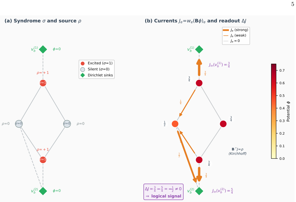
The central claim is Proposition 1: for the syndrome graph with two boundary sinks at equal potential, the net current drained between the sinks equals the sum over excited detectors of (1−2χ_v), where χ is the unique harmonic coordinate taking value 0 on one code boundary and 1 on the other. Because the graph is one-dimensional, the edge current generated by the discrete Poisson equation has no co-exact (circulating) part; it is a pure gradient, so no component of the current carries the logical class. Instead the logical class is carried by the relative cohomology class H^1(G,∂G;Z2): the learned edge weights fix which harmonic representative χ is used, and the syndrome is measured against
What carries the argument
The construction uses discrete exterior calculus on the syndrome graph: the signed incidence matrix B acts as the discrete exterior derivative, and the weighted graph Laplacian L=B^T diag(w)B is the discrete Hodge Laplacian. The decoder solves the discrete Gauss law Lφ=σ with Dirichlet boundary conditions, and then evaluates the logical signal as the difference of currents entering two boundary sinks. Proposition 1 identifies this sink-current difference with the pairing Σ_{σ_v=1}(1−2χ_v), where χ is the harmonic coordinate solving Lχ=0 in the interior with boundary values 0 and 1 on the two sinks. The learned weights w deform χ; the readout itself has no free parameters.
Load-bearing premise
The load-bearing premise is that the circuit-level syndrome graph has exactly one relative homology class carrying the logical information, so that a single harmonic coordinate χ separating the two boundary sinks is sufficient; if the graph carried additional nonlocal relative classes, the scalar pairing would miss part of the logical signal.
What would settle it
Compute the first relative homology group H1(G,∂G;Z2) of the actual circuit-level detector-error-model graph for the distance-7 code: if its dimension is greater than one, the single-coordinate pairing cannot capture all logical information. A direct experimental check is to evaluate Eq. (9) at converged weights on every test syndrome and compare the sign of s with the ground-truth logical label; any syndrome whose label is not determined by s would falsify the claim that the pairing is the logical signal.
If this is right
- A single boundary sink is not just a worse readout: it removes the topological object being measured, since no harmonic function can separate two boundaries that have been merged.
- Because the logical signal is one-dimensional, a single closed-form scalar saturates the information a full-field readout can access; at distance 7 it significantly outperforms the single-sink current pool.
- For a code with k logical qubits, the same construction gives 2k boundary sinks and k independent harmonic coordinates, one per logical boundary pair, with no other architectural change.
- The decoder is not intended to replace minimum-weight perfect matching; its value is an exact, interpretable readout that separates the logical invariant from the learned metric.
- The signed vote 1−2χ_v for each excited detector runs from +1 to −1 across the code, so the readout can be viewed as a convex vote along the learned harmonic coordinate.
Where Pith is reading between the lines
- A step the paper does not take but its identity allows: because Prop. 1 makes the readout independent of learned readout parameters, one could train only the edge-weight metric and evaluate the logical signal exactly at inference, eliminating the need for a Poisson solve for φ and solving only for χ.
- The same two-sink pairing should transfer to any planar code with two opposing boundary components and one logical qubit—for example lattice-surgery patches or planar codes with holes—without retraining the architecture.
- If the relative homology group of a realistic circuit-level syndrome graph ever contains more than one nonlocal class, the scalar pairing would be incomplete; checking dim H1(G,∂G;Z2) directly on a detector-error-model graph would settle whether the single-harmonic-coordinate assumption holds.
- The empirical parity between the two-sink scalar and the full-field readout suggests that the logical signal is genuinely one-dimensional under circuit-level noise; a testable prediction is that any readout that projects onto the harmonic representative will discard no information, and that the advantage over single-sink readouts should grow with code distance.
Editorial analysis
A structured set of objections, weighed in public.
Referee Report
Summary. The paper proposes a physics-informed GNN decoder for the rotated surface code in which a weighted graph Laplacian is solved as a discrete Poisson equation, with the syndrome as the source. Four readouts are compared: a full-field edge-current pool, a two-sink net-current readout, a node-potential readout, and a diffusion readout. The central theoretical claim is Proposition 1: for two Dirichlet boundary sinks held at equal potential, the net current drained between them equals the pairing Σ_{v:σ_v=1}(1−2χ_v), where χ is the harmonic coordinate with boundary values 0 and 1. The paper interprets this pairing as the complete logical-error signal, evaluated exactly and without learned readout parameters. Empirically, on d=5 and d=7 circuit-level depolarising noise, the two-sink readout ties the best full-field readout and exceeds the single-sink current pool at d=7.
Significance. If taken as an interpretable and approximate linear statistic, the work has genuine value. Proposition 1 is a correct and clean discrete Green's identity, and the controlled same-split, multi-seed ablation is a strength. The paper is also commendably explicit about its limitations, including the residual of the truncated Jacobi solve and the fact that the decoder does not surpass MWPM. However, the manuscript's headline claims—that the readout is the exact topological pairing, that it is evaluated in closed form with no learned readout parameters, and that its parity with full-field readouts is predicted by the one-dimensional relative homology of the syndrome graph—are not supported by the text as written. These issues are central to the paper's stated contribution and require substantive revision.
major comments (3)
- [§II D–E, Eq. (9)] The premise that dim H1(G,∂G;Z2)=k=1 for the circuit-level DEM graph is unsupported and, for a graph, generically false. For a connected graph with two boundary vertices, rank H1(G,∂G;Z2)=|E|−|V|+2, i.e. the ordinary cycle rank plus one. The DEM graph for d=5, r=5 has 120 detector nodes plus 2 sinks and many independent cycles; local cycles are nonzero relative classes because the graph is treated as a 1-dimensional complex with no 2-cells. Thus χ is only one harmonic coordinate among many, and s is one linear projection of the syndrome, not "the" topological pairing whose dimension is fixed by k. The empirical parity with ϕ-readout is therefore not explained by the stated k=1 argument. The authors must either prove a special property of the actual DEM graph that makes the asserted dimension hold, or substantially weaken the topological-completeness claims.
- [Abstract, §III G, Appendix B] The abstract and §III G state that the pairing is "evaluated exactly and in closed form, with no learned readout parameters." This is contradicted by Appendix B: at the operating budget K_J=25 the interior residual is 0.150±0.028 at d=5, so the implemented quantity is s^(25), a truncated Jacobi approximation, not the exact Proposition 1 quantity. Additionally, the small MLP that maps s to a logit in §III G is a learned readout parameter. The proposition itself is exact at the fixed point, but the implementation never reaches it; the distinction between s^(25) and s^(∞) is not cosmetic because the calibration is trained on s^(25). The claims should be revised to describe the readout as an approximate, learned-calibrated statistic, or the solver should be run to convergence for all reported results.
- [§VI A, §VI C, Table II] The generalization statement that k>1 codes require 2k sinks and that the readout measures generators of H1(G,∂G;Z2) inherits the same problem: the graph's relative homology contains many local cycles, so the proposed construction does not, as written, isolate exactly one logical generator per logical qubit. The d=7 comparison with the ϕ-readout is also presented as a tie, but it hinges on excluding one seed with a reported dead start; with all five seeds the paired difference is not significant. This is acceptable as a hypothesis, but it does not constitute evidence for the claim that a single scalar "saturates" the logical information. Please rephrase the interpretation to be explicitly empirical rather than a consequence of the relative-homology dimension.
minor comments (5)
- [§II D] The notation H1(G,∂G;Z2) is used for both homology and cohomology; the distinction matters because the harmonic coordinate χ is a 0-cochain and d0χ is a 1-cochain. Consider introducing separate notation or a clarifying sentence.
- [§III H, Eq. (18)] The diffusion update u^{(k+1)} = u^{(k)} − Δt L u^{(k)} integrates ˙u = −L u, but the sign convention in the text appears inconsistent with the preceding sentence. Please check and unify.
- [Table II] The Wilcoxon p-values are reported as p=0.06 and p=0.13, while the text says the two-sink advantage is positive on all five seeds. Given the small sample, the wording "genuine and significant" for t=4.1 should be tempered by the non-significant Wilcoxon result.
- [General] The paper does not state whether code or data will be released. Given the emphasis on reproducibility and the controlled ablation, a code/data availability statement would be valuable.
- [§V A] The logical-axis determination uses the true labels to select the axis. This is a legitimate zero-training heuristic, but it should be described as label-informed rather than "zero-training," since the labels are used for axis selection.
Circularity Check
No circular derivation: Prop. 1 is a genuine algebraic identity; the main risk is an unproved homology-counting claim, which is a correctness/foundational issue, not an equivalence-to-input.
full rationale
The paper's central result, Proposition 1 (Eqs. 8-9), is a self-contained Green's-identity calculation: for any fixed positive edge metric w, the two-sink Dirichlet solution phi and the auxiliary harmonic function chi with boundary values 0 and 1 give s = sum_{sigma_v=1}(1-2chi_v) as the net sink current. The proof uses only symmetry of L(w)=B^T diag(w)B and the Dirichlet boundary conditions; it does not invoke the labels, the learned calibration, or any fitted readout parameter. For fixed w, the statement is parameter-free and has independent mathematical content, so it is not circular. The GNN edge-weight MLP and the final calibration MLP are trained on labels, but that is ordinary supervised learning on held-out splits, not a case where the predicted quantity is the fitted input. The main caveat is in Section II D-E: the paper asserts that dim H_1(G,dG;Z_2) equals k and that one harmonic coordinate captures the complete logical signal ('the logically relevant subspace is the homology relative to the code boundary... whose dimension is the number k of logical qubits'). For a circuit-level DEM graph, which is a 1-dimensional complex with many independent local cycles, this identification is not automatic and is likely false; the scalar s may be one learned projection rather than 'the' topological invariant. That is a serious correctness/foundational risk, and the abstract's strongest claim should be qualified, but it is not a circular reduction of the paper's outputs to its inputs. No load-bearing self-citation chain or uniqueness argument imported from the authors is present.
Axiom & Free-Parameter Ledger
free parameters (4)
- GINE encoder and edge-weight MLP parameters
- Calibration MLP parameters mapping s to logit
- Logical-axis and boundary-partition choice
- Jacobi iteration budget K_J and diffusion budget K_D, Δt_max =
K_J=25, K_D=15, Δt_max=0.5
axioms (6)
- standard math Weighted graph Laplacian L=B^T diag(w)B and discrete Gauss law B^T J=ρ hold exactly on the syndrome graph
- standard math The syndrome graph is a 1-dimensional simplicial complex with no 2-cells, so the Hodge decomposition of 1-forms has only exact and harmonic parts
- standard math Green's identity and symmetry of the weighted Laplacian give Proposition 1
- domain assumption The syndrome graph's relative cohomology H^1(G,∂G;Z2) is one-dimensional and captures the logical class of the Z-bar operator
- domain assumption Circuit-level DEM error mechanisms map to edges of a syndrome graph whose two selected boundary sinks correspond to the two physical boundaries linked by Z-bar
- domain assumption p=0.005 is a well-resolved regime where readout comparisons are meaningful
Cite this review
Pith. "Pith review of Physics-Informed Graph-Neural Decoding of the Surface Code: the Logical Signal as an Exact Topological Pairing." pith.science (2026). https://pith.science/paper/QBQ443YD
@misc{pith2026260720060,
  author       = {Pith},
  title        = {Pith review of: Physics-Informed Graph-Neural Decoding of the Surface Code: the Logical Signal as an Exact Topological Pairing},
  year         = {2026},
  howpublished = {\url{https://pith.science/paper/QBQ443YD}},
  note         = {Machine review of arXiv:2607.20060}
}
read the original abstract
We develop a physics-informed graph neural network (GNN) decoder for the surface code that solves a discrete Poisson equation on the syndrome graph, with the syndrome as the charge source. We compare four readout architectures for extracting the logical-error probability: a potential-based readout that maps the Poisson field through a multilayer perceptron, two current-based readouts under single- and two-sink Dirichlet boundary conditions, and a diffusion-based variant. Comparing these, we show that the solver's edge current is a pure gradient flow whose harmonic (circulating) part vanishes identically. The logical signal therefore cannot be read as a component of the current itself; it is instead a topological pairing between the syndrome and a boundary-fixed harmonic coordinate that distinguishes the two code boundaries linked by the logical operator. We prove that this pairing is evaluated exactly and in closed form, with no learned readout parameters, as the net current drained between the two boundary sinks. On the rotated surface code under circuit-level depolarising noise, this single closed-form scalar matches the best full-field readout and, at larger code distance, significantly exceeds the single-sink current pool, so that isolating the pairing helps more, not less, as the field grows larger and sparser. The decoder is not intended to surpass minimum-weight perfect matching, near-optimal for this noise model; its contribution is an interpretable characterisation of the logical signal itself.
Figures




Reference graph
Works this paper leans on
-
[1]
B. M. Terhal, Quantum error correction for quantum memories, Reviews of Modern Physics87, 307 (2015)
2015
-
[2]
A. Y. Kitaev, Fault-tolerant quantum computation by anyons, Ann. Phys.303, 2 (2003)
2003
-
[3]
Dennis, A
E. Dennis, A. Kitaev, A. Landahl, and J. Preskill, Topological quantum memory, J. Math. Phys.43, 4452 (2002)
2002
-
[4]
Edmonds, Paths, trees, and flowers, Can
J. Edmonds, Paths, trees, and flowers, Can. J. Math.17, 449 (1965)
1965
-
[5]
Nishimori, Internal energy, specific heat and correlation function of the bond-random Ising model, Prog
H. Nishimori, Internal energy, specific heat and correlation function of the bond-random Ising model, Prog. Theor. Phys. 66, 1169 (1981)
1981
-
[6]
Torlai and R
G. Torlai and R. G. Melko, Neural decoder for topological codes, Phys. Rev. Lett.119, 030501 (2017)
2017
-
[7]
Varsamopoulos, B
S. Varsamopoulos, B. Criger, and K. Bertels, Decoding small surface codes with feedforward neural networks, Quantum Sci. Technol.3, 015004 (2017)
2017
-
[8]
Krastanov and L
S. Krastanov and L. Jiang, Deep neural network probabilistic decoder for stabilizer codes, Sci. Rep.7, 11003 (2017)
2017
-
[9]
Baireuther, T
P. Baireuther, T. E. O’Brien, B. Tarasinski, and C. W. J. Beenakker, Machine-learning-assisted correction of correlated qubit errors in a topological code, Quantum2, 48 (2018)
2018
-
[10]
Maskara, A
N. Maskara, A. Dua, and M. D. Lukin, Advantages of versatile neural-network decoding for topological codes, Phys. Rev. A99, 052351 (2019)
2019
-
[11]
Meinerz, C.-Y
K. Meinerz, C.-Y. Park, and S. Trebst, Scalable neural decoder for topological surface codes, Phys. Rev. Lett.128, 080505 (2022)
2022
-
[12]
J. Bauschet al., Learning to decode the surface code with a recurrent, transformer-based neural network (2023), arXiv:2310.05900
Pith/arXiv arXiv 2023
-
[13]
R. W. J. Overwater, M. Babaie, and F. Sebastiano, Neural-network decoders for quantum error correction using surface codes: A space exploration of the implementation cost-performance trade-offs, IEEE Trans. Quantum Eng.3, 1 (2022)
2022
-
[14]
Lange, P
M. Lange, P. Havstr¨ om, B. Srivastava, I. Bengtsson, V. Bergentall, K. Hammar, O. Heuts, E. van Nieuwenburg, and M. Granath, Data-driven decoding of quantum error correcting codes using graph neural networks, Phys. Rev. Res.7, 023181 (2025)
2025
-
[15]
S. Gicev, L. C. L. Hollenberg, and M. Usman, A scalable and fast artificial neural network syndrome decoder for a chain of surface codes (2023), arXiv:2110.11390
Pith/arXiv arXiv 2023
-
[16]
Joo, Decoding the surface code with a spatio-temporal transformer, EPJ Quantum Technology13, 52 (2026)
R. Joo, Decoding the surface code with a spatio-temporal transformer, EPJ Quantum Technology13, 52 (2026). 19 0 100 200 300 400 500 600 Epoch 0.5 0.6 0.7 0.8 0.9 1.0Validation AUC J-readout (single-sink) J-readout (two-sink harmonic) -readout Diffusion-readout FIG. 6. Validation AUC vs. epoch for the four readouts atd= 5,p= 0.005, under the common protoco...
2026
-
[17]
Belkin and P
M. Belkin and P. Niyogi, Laplacian eigenmaps and spectral techniques for embedding and clustering, NIPS (2001)
2001
-
[18]
X. Zhu, Z. Ghahramani, and J. Lafferty, Semi-supervised learning using gaussian fields and harmonic functions, ICML (2003)
2003
-
[19]
D. Zhou, O. Bousquet, T. N. Lal, J. Weston, and B. Sch¨ olkopf, Learning with local and global consistency, inNIPS(2004)
2004
-
[20]
A. G. Fowler, J. M. Martinis, A. Megrant, and J. Kelly, Surface codes: Towards practical large-scale quantum computation, Phys. Rev. A86, 032324 (2012)
2012
-
[21]
Gidney, Stim: a fast stabilizer circuit simulator, Quantum5, 497 (2021)
C. Gidney, Stim: a fast stabilizer circuit simulator, Quantum5, 497 (2021)
2021
-
[22]
O. Higgott and C. Gidney, Sparse blossom: correcting a million errors per core second with minimum-weight matching (2023), arXiv:2303.15933
Pith/arXiv arXiv 2023
-
[23]
A. N. Hirani,Discrete exterior calculus, Ph.D. thesis, California Institute of Technology (2003)
2003
-
[24]
M. Desbrun, E. Kanso, and Y. Tong, Discrete differential forms for computational modeling, SIGGRAPH Courses 10.1145/1198555.1198666 (2005)
arXiv 2005
-
[25]
W. Hu, B. Hou, J. Liu, and J. Leskovec, Strategies for pre-training graph neural networks, inICLR(2020)
2020
-
[26]
Y. Li, D. Tarlow, M. Brockschmidt, and R. Zemel, Gated graph sequence neural networks, ICLR (2016)
2016
-
[27]
D. P. Kingma and J. Ba, Adam: A method for stochastic optimization, ICLR (2015)
2015
-
[28]
W. Zhong, O. Shtanko, and R. Movassagh, Advantage of quantum neural networks as quantum information decoders (2024), arXiv:2401.06300 [quant-ph]
Pith/arXiv arXiv 2024
-
[29]
Frankel,The Geometry of Physics: An Introduction, 3rd ed
T. Frankel,The Geometry of Physics: An Introduction, 3rd ed. (Cambridge University Press, 2011)
2011
discussion (0)
Sign in with ORCID, Apple, or X to comment. Anyone can read and Pith papers without signing in.