REVIEW 2 major objections 6 minor 28 references
This paper shows that a graph neural network built from polynomial layers can be attributed exactly by Aumann–Shapley path integration with a fixed, architecture-determined number of evaluation points.
Reviewed by Pith at T0; open to challenge. T0 means a machine referee read the full paper against a public rubric. the ladder, T0–T4 →
T0 review · deepseek-v4-flash
2026-08-01 08:28 UTC pith:UVBGDRBQ
load-bearing objection The exact-integration theory is sound; the headline fidelity result is a confounded system comparison. the 2 major comments →
A Polynomial Architecture-Attribution Co-Design Framework for Exact Aumann-Shapley Attribution in GNNs
The pith
A machine-rendered reading of the paper's core claim, the machinery that carries it, and where it could break.
Core claim
The central claim is Theorem 1: for a PolyGIN with L polynomial transformation blocks, the scalar logit is a multivariate polynomial in the input features of degree at most 2^L; hence each partial derivative along the straight-line path has degree at most 2^L − 1. Standard Gauss–Legendre quadrature with m = 2^(L−1) points integrates such a univariate polynomial exactly. The result converts integrated-gradients-style attribution from a resolution-dependent numerical approximation into a fixed finite computation with a deterministic evaluation budget, while additive node-level aggregation (summing feature attributions per node) preserves the completeness identity that the feature attributions
What carries the argument
PolyGIN, a message-passing network built so that all steps are linear except a quadratic polynomial activation z + θ⊙z²; graph-isomorphism-style sum aggregation, linear projections, and a learnable diagonal scaling are linear, so compositions keep the input-to-logit map polynomial. The load-bearing identity is the Gauss–Legendre exactness property: an m-point rule integrates polynomials of degree up to 2m − 1 exactly. Combined with the degree bound for PolyGIN, this fixes m = 2^(L−1) and eliminates quadrature truncation error.
Load-bearing premise
Every operation that touches the attributed score must be polynomial or linear in the input features, and the attribution must be taken on the pre-softmax logit along a fixed straight-line path from a chosen baseline; introduce a ReLU, batch norm, softmax, or attention softmax anywhere and the degree bound—and with it the exactness guarantee—no longer holds.
What would settle it
Train a four-block PolyGIN, compute APEX attributions with the prescribed eight Gauss–Legendre points, and compare against a high-resolution numerical integration (say 512-point Gauss–Legendre or Simpson) on the same model. If the two attribution vectors differ by more than floating-point roundoff, or if the completeness error exceeds machine precision for any input, Theorem 1 fails for that model. A simpler check: insert one ReLU activation into the last block and measure the completeness error of an eight-point rule—it should jump well above FP32 precision.
If this is right
- For any fixed-depth PolyGIN, exact Aumann–Shapley attribution costs exactly 2^(L−1) forward-backward evaluations, independent of any user-chosen integration resolution.
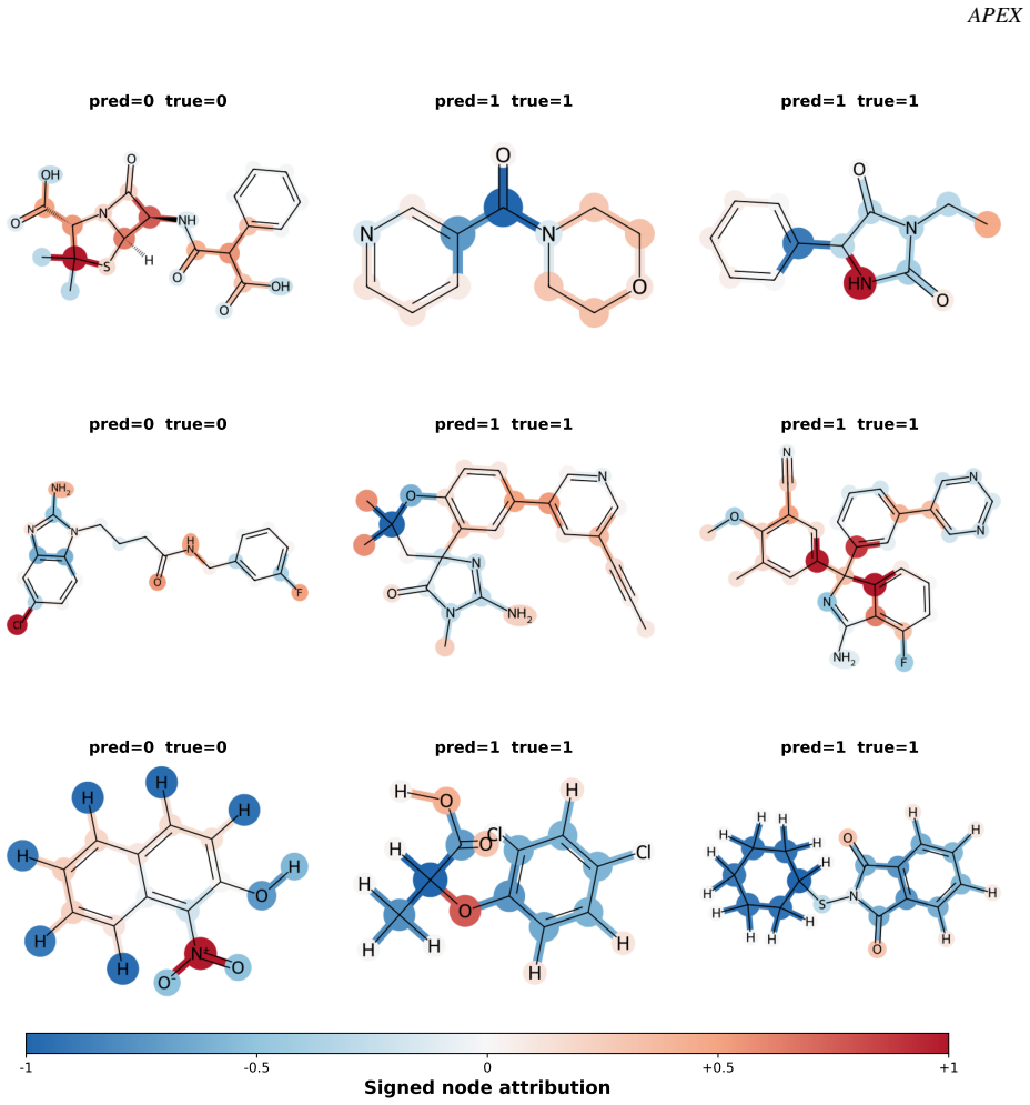
- Completeness holds to floating-point precision: feature attributions sum to the logit difference, and signed node-level attributions decompose a prediction into supporting and opposing evidence.
- No convergence sweep or error tolerance is needed; truncation error from path discretization is eliminated under the polynomial assumptions.
- The polynomial constraint does not cost much accuracy: on the five benchmarks tested, PolyGIN stays within about one percentage point of a standard graph isomorphism network.
- Fidelity experiments (necessary and sufficient subsets) favor the complete framework over several post-hoc explainers on the evaluated datasets.
Where Pith is reading between the lines
- The co-design principle could transfer to other continuous attribution frameworks: any path integral whose integrand is polynomial in the path parameter inherits an exact finite quadrature budget, so other baselines or paths may be handled with adjusted degree bounds.
- The exponential degree growth (2^L) caps practical depth; the paper uses four blocks, and deeper polynomial networks may need additional scaling or regularization to remain stable.
- The exactness guarantee is tied to pre-softmax logits; users attributing probabilities or using batch norm, ReLU, or attention softmax must accept the same quadrature error the framework removes. A testable extension is to design polynomial analogues of attention or normalization that keep the degree bound.
- The nearly identical fidelity of numerical integrated gradients and APEX on the same PolyGIN backbone suggests the fidelity gain over other explainers comes from the architecture-plus-attribution combination rather than from exactness alone; the paper argues this in an appendix.
Editorial analysis
A structured set of objections, weighed in public.
Referee Report
Summary. The paper proposes APEX, a co-design framework pairing a polynomial GNN architecture (PolyGIN) with exact Aumann–Shapley attribution. PolyGIN replaces non-polynomial components with linear operations and the polynomial activation σ_poly(z)=z+θ⊙z², so the pre-softmax logit is a multivariate polynomial in the input features. Theorem 1 gives a degree bound of 2^L for the logit, hence a degree bound of 2^L−1 for the path integrand; Gauss–Legendre quadrature with m=2^{L−1} points then evaluates the attribution integral exactly. Feature-level attributions are summed into signed node-level scores with completeness preserved. Experiments on five graph benchmarks compare predictive accuracy, fidelity, completeness error, and runtime. The theoretical derivation is self-contained and the induction in Theorem 1 is correct; the main weakness is the empirical fidelity comparison, which does not clearly control the attributed backbone.
Significance. If the claims hold, the paper contributes a clean and useful result: a class of GNNs for which Integrated-Gradients-style path integrals are evaluated exactly with a fixed, architecture-determined number of forward–backward evaluations. The proof is elementary but rigorous, and the empirical completeness-error experiment (Figure 5) directly confirms the predicted 8-point exactness for a 4-block PolyGIN. The paper also usefully separates algebraic exactness from 1-WL expressivity in Appendix B. However, the practical relevance advertised in the abstract depends on the fidelity experiments, and those experiments are currently confounded by inadequate reporting of the backbone used for each explainer. The scope is also narrower than the title suggests: exactness holds only for polynomial architectures and pre-softmax logits, a limitation the authors do acknowledge in the conclusion.
major comments (2)
- [§4.3, Figures 3–4, Appendix D, Figures 6–7] The main fidelity comparison does not state which trained backbone each explainer is evaluated on. Table 1 reports only GIN vs. PolyGIN accuracy, and §4.3 merely says 'all methods' are evaluated on correctly classified test graphs. Appendix D reveals that when all explainers are evaluated on the same trained PolyGIN models, numerical IG achieves fidelity 'nearly identical' to APEX. This strongly implies that the headline Figures 3–4 compare APEX on PolyGIN against baselines on GIN. If so, the claimed fidelity advantage may be due to the architecture, not to exact Gauss–Legendre quadrature. Please present the same-backbone comparison as the primary fidelity result, or explicitly reframe Figures 3–4 as a system-level comparison of (PolyGIN+APEX) versus (GIN+baseline) and add a table stating the backbone used for every method.
- [§3.1, §4.3, Eqs. (10), (13), (14)] APEX attributes the pre-softmax logit f_c, but the fidelity metrics are computed on softmax probabilities p_c after masking/retaining nodes. The paper never justifies that a positive attribution to the logit f_c implies a corresponding change in p_c, since p_c depends on all logits through the softmax denominator. The monotonic link may hold approximately in practice but is not guaranteed. This mismatch is load-bearing for the empirical fidelity claim: an exact logit decomposition can rank nodes differently from a probability-based fidelity protocol. Please either report fidelity based on the attributed logit as well, or state and justify the assumption that logit and probability rankings agree under the perturbation protocol.
minor comments (6)
- [Title and Abstract] The title and abstract claim 'exact Aumann–Shapley attribution in GNNs,' but the exactness is conditional on the polynomial architecture and on attributing pre-softmax logits. The conclusion states this explicitly. Please qualify the title/abstract, e.g., 'in polynomial GNNs' or 'under polynomial architectures.'
- [§4.4, Eq. (9)] The notation 'm=2^{L−1}' and the degree bound '2^L−1' are visually confusable in plain text, and several sentences render '2 L−1' without superscripts. Use consistent typesetting, e.g., m=2^{L-1} and deg = 2^L-1.
- [Figures 3–4] No variance/error bars are shown for the fidelity results, even though Table 1 reports ten seeds. State whether the fidelity curves are averages over seeds and report standard deviations or at least a seed count.
- [Table 3] The Mutagenicity label mapping in Table 3 (Label 1 = Non-mutagenic, Label 0 = Mutagenic) is the opposite of the common convention for this dataset. Please verify the encoding and explicitly define the labels used in the visualization; otherwise the qualitative discussion of 'mutagenic' vs. 'non-mutagenic' examples may mislead readers.
- [Appendix D] The same-backbone control is important and currently appears only in an appendix. Move a condensed version into the main text or at least add a sentence in §4.3 stating explicitly that a same-backbone control is provided and what it shows.
- [§5] There is a duplicated phrase in the final sentence of the completeness-error discussion: '...consistent with floating-point roundoff rather than quadrature truncation error, rather than from approximation error...' Remove the redundancy.
Circularity Check
No significant circularity: the APEX exactness result is derived from architecture definitions and classical Gauss-Legendre quadrature, not from its own outputs.
full rationale
The central derivation is self-contained and non-circular. Theorem 1 is a direct induction on Definitions 1-3: aggregation, linear projection, and PolyScaleNorm are linear; PolyActivation z + theta⊙z^2 at most doubles degree, so after L blocks the logit has degree at most 2^L and any partial derivative has degree at most 2^L-1. The quadrature budget m = 2^{L-1} follows from the classical Gauss-Legendre exactness condition (m points integrate degree at most 2m-1), and Eq. (10) is just the mapped GL rule applied to Eq. (2). Node-level completeness (Eq. 12) is summation of feature attributions. Nothing is fitted and then called a prediction: the 8-point result in Fig. 5 is computed from the stated L=4 and checked against FP32 completeness error, not used to set a constant. The paper cites no prior work by its own authors, so no self-citation chain is load-bearing; the Hesse et al. and Gauss-Legendre citations are external standard results. Appendix D provides a same-backbone control and notes that numerical IG on PolyGIN is 'nearly identical' to APEX, which is a consistency check of the same Aumann-Shapley quantity, not circularity. The Conclusion explicitly limits exactness to polynomial logits and excludes ReLU/softmax/batchnorm operations, showing the claim is conditional rather than definitionally forced to fit observed data. The possible fidelity-comparison confound between different backbones is an experimental-design concern, not a circularity in the derivation.
Axiom & Free-Parameter Ledger
axioms (5)
- standard math An m-point Gauss–Legendre rule exactly integrates every polynomial of degree at most 2m−1.
- domain assumption The attributed model output is the pre-softmax logit, with no non-polynomial output layer in the path being integrated.
- domain assumption All PolyGIN operations (GIN sum aggregation, linear maps, PolyScaleNorm, PolyActivation) preserve polynomial dependence on input features, for each fixed graph topology.
- domain assumption Attribution is taken along the straight-line path from a baseline input to the target input.
- domain assumption For the WL expressivity analysis: countable input feature universe, bounded node degrees, layer-wise injectivity (Assumption 1), and injective graph-level readout.
invented entities (3)
-
PolyGIN
independent evidence
-
PolyActivation σ_poly(z)=z+θ⊙z²
no independent evidence
-
PolyScaleNorm
no independent evidence
read the original abstract
We study feature-level and node-level explanations for graph neural networks (GNNs) through the lens of Aumann-Shapley attribution. Path-integral methods such as Integrated Gradients provide an axiomatic formulation of attribution, but their practical use in deep GNNs typically relies on finite-sample numerical approximations to the path integral, requiring a trade-off between quadrature error and computational cost. This paper proposes APEX, a model-attribution co-design framework that makes the attribution integral exactly computable under a polynomial GNN architecture. The key component is PolyGIN, a GIN-style graph network whose message-passing, normalization, and transformation operations preserve a bounded multivariate polynomial form for scalar model scores, such as pre-softmax logits. We show that, for a PolyGIN with $L$ polynomial transformation blocks, the derivative along the attribution path has degree at most $2^L-1$. Therefore, Gauss--Legendre quadrature can evaluate the Aumann--Shapley path integral exactly, up to floating-point precision, with $2^{L-1}$ deterministic evaluation points. The resulting attributions can be computed at the feature level and then aggregated into node-level scores while preserving completeness. Experiments on synthetic and real-world graph benchmarks show that PolyGIN maintains competitive predictive performance, while the complete APEX framework achieves higher attribution fidelity than the compared baselines and substantially reduces the number of evaluations required for path integration.
Figures


Reference graph
Works this paper leans on
-
[1]
Graph neural networks in recommender systems: a survey.ACM Computing Surveys, 55(5):1–37, 2022
Shiwen Wu, Fei Sun, Wentao Zhang, Xu Xie, and Bin Cui. Graph neural networks in recommender systems: a survey.ACM Computing Surveys, 55(5):1–37, 2022
2022
-
[2]
Graph neural networks for social recommendation
Wenqi Fan, Yao Ma, Qing Li, Yuan He, Eric Zhao, Jiliang Tang, and Dawei Yin. Graph neural networks for social recommendation. InThe world wide web conference, pages 417–426, 2019
2019
-
[3]
Graph convolutional networks for text classification
Liang Yao, Chengsheng Mao, and Yuan Luo. Graph convolutional networks for text classification. InProceedings of the AAAI conference on artificial intelligence, volume 33, pages 7370–7377, 2019
2019
-
[4]
Dejun Jiang, Zhenxing Wu, Chang-Yu Hsieh, Guangyong Chen, Ben Liao, Zhe Wang, Chao Shen, Dongsheng Cao, Jian Wu, and Tingjun Hou. Could graph neural networks learn better molecular representation for drug dis- covery? a comparison study of descriptor-based and graph-based models.Journal of cheminformatics, 13(1):12, 2021. 10 APEX
2021
-
[5]
Neural message passing for quantum chemistry
Justin Gilmer, Samuel S Schoenholz, Patrick F Riley, Oriol Vinyals, and George E Dahl. Neural message passing for quantum chemistry. InInternational conference on machine learning, pages 1263–1272. Pmlr, 2017
2017
-
[6]
Axiomatic attribution for deep networks
Mukund Sundararajan, Ankur Taly, and Qiqi Yan. Axiomatic attribution for deep networks. InInternational conference on machine learning, pages 3319–3328. PMLR, 2017
2017
-
[7]
Princeton University Press, 2015
Robert J Aumann and Lloyd S Shapley.Values of non-atomic games. Princeton University Press, 2015
2015
-
[8]
The many shapley values for model explanation
Mukund Sundararajan and Amir Najmi. The many shapley values for model explanation. InInternational conference on machine learning, pages 9269–9278. PMLR, 2020
2020
-
[9]
Explainability in graph neural networks: A taxonomic survey.IEEE transactions on pattern analysis and machine intelligence, 45(5):5782–5799, 2022
Hao Yuan, Haiyang Yu, Shurui Gui, and Shuiwang Ji. Explainability in graph neural networks: A taxonomic survey.IEEE transactions on pattern analysis and machine intelligence, 45(5):5782–5799, 2022
2022
-
[10]
Gnnexplainer: Generating explanations for graph neural networks.Advances in neural information processing systems, 32, 2019
Zhitao Ying, Dylan Bourgeois, Jiaxuan You, Marinka Zitnik, and Jure Leskovec. Gnnexplainer: Generating explanations for graph neural networks.Advances in neural information processing systems, 32, 2019
2019
-
[11]
Parameter- ized explainer for graph neural network.Advances in neural information processing systems, 33:19620–19631, 2020
Dongsheng Luo, Wei Cheng, Dongkuan Xu, Wenchao Yu, Bo Zong, Haifeng Chen, and Xiang Zhang. Parameter- ized explainer for graph neural network.Advances in neural information processing systems, 33:19620–19631, 2020
2020
-
[12]
On explainability of graph neural networks via subgraph explorations
Hao Yuan, Haiyang Yu, Jie Wang, Kang Li, and Shuiwang Ji. On explainability of graph neural networks via subgraph explorations. InInternational conference on machine learning, pages 12241–12252. PMLR, 2021
2021
-
[13]
Flowx: Towards explainable graph neural networks via message flows.IEEE Transactions on Pattern Analysis and Machine Intelligence, 46(7):4567–4578, 2023
Shurui Gui, Hao Yuan, Jie Wang, Qicheng Lao, Kang Li, and Shuiwang Ji. Flowx: Towards explainable graph neural networks via message flows.IEEE Transactions on Pattern Analysis and Machine Intelligence, 46(7):4567–4578, 2023
2023
-
[14]
Explainability methods for graph convolutional neural networks
Phillip E Pope, Soheil Kolouri, Mohammad Rostami, Charles E Martin, and Heiko Hoffmann. Explainability methods for graph convolutional neural networks. InProceedings of the IEEE/CVF conference on computer vision and pattern recognition, pages 10772–10781, 2019
2019
-
[15]
A value for n-person games
Lloyd S Shapley et al. A value for n-person games. 1953
1953
-
[16]
Fast axiomatic attribution for neural networks.Advances in Neural Information Processing Systems, 34:19513–19524, 2021
Robin Hesse, Simone Schaub-Meyer, and Stefan Roth. Fast axiomatic attribution for neural networks.Advances in Neural Information Processing Systems, 34:19513–19524, 2021
2021
-
[17]
On the expressive power of deep polynomial neural networks
Joe Kileel, Matthew Trager, and Joan Bruna. On the expressive power of deep polynomial neural networks. Advances in neural information processing systems, 32, 2019
2019
-
[18]
P-nets: Deep polynomial neural networks
Grigorios G Chrysos, Stylianos Moschoglou, Giorgos Bouritsas, Yannis Panagakis, Jiankang Deng, and Stefanos Zafeiriou. P-nets: Deep polynomial neural networks. InProceedings of the IEEE/CVF Conference on Computer Vision and Pattern Recognition, pages 7325–7335, 2020
2020
-
[19]
Convolutional neural networks on graphs with fast localized spectral filtering.Advances in neural information processing systems, 29, 2016
Michaël Defferrard, Xavier Bresson, and Pierre Vandergheynst. Convolutional neural networks on graphs with fast localized spectral filtering.Advances in neural information processing systems, 29, 2016
2016
-
[20]
How powerful are graph neural networks? In International Conference on Learning Representations, 2019
Keyulu Xu, Weihua Hu, Jure Leskovec, and Stefanie Jegelka. How powerful are graph neural networks? In International Conference on Learning Representations, 2019
2019
-
[21]
Calculation of gauss quadrature rules.Mathematics of computation, 23(106):221–230, 1969
Gene H Golub and John H Welsch. Calculation of gauss quadrature rules.Mathematics of computation, 23(106):221–230, 1969
1969
-
[22]
Robust design with arbitrary distributions using gauss-type quadrature formula.Structural and Multidisciplinary Optimization, 39(3):227–243, 2009
Sang Hoon Lee, Wei Chen, and Byung Man Kwak. Robust design with arbitrary distributions using gauss-type quadrature formula.Structural and Multidisciplinary Optimization, 39(3):227–243, 2009
2009
-
[23]
Graphframex: Towards systematic evaluation of explainability methods for graph neural networks
Kenza Amara, Rex Ying, Zitao Zhang, Zhihao Han, Yinan Shan, Ulrik Brandes, Sebastian Schemm, and Ce Zhang. Graphframex: Towards systematic evaluation of explainability methods for graph neural networks. arXiv preprint arXiv:2206.09677, 2022
Pith/arXiv arXiv 2022
-
[24]
Towards robust fidelity for evaluating explainability of graph neural networks
Xu Zheng, Farhad Shirani, Tianchun Wang, Wei Cheng, Zhuomin Chen, Haifeng Chen, Hua Wei, and Dongsheng Luo. Towards robust fidelity for evaluating explainability of graph neural networks. InInternational Conference on Learning Representations, volume 2024, pages 12250–12275, 2024
2024
-
[25]
Cambridge university press, 2003
Endre Süli and David F Mayers.An introduction to numerical analysis. Cambridge university press, 2003
2003
-
[26]
Moleculenet: a benchmark for molecular machine learning.Chemical science, 9(2):513–530, 2018
Zhenqin Wu, Bharath Ramsundar, Evan N Feinberg, Joseph Gomes, Caleb Geniesse, Aneesh S Pappu, Karl Leswing, and Vijay Pande. Moleculenet: a benchmark for molecular machine learning.Chemical science, 9(2):513–530, 2018
2018
-
[27]
Derivation and validation of toxicophores for mutagenicity prediction.Journal of medicinal chemistry, 48(1):312–320, 2005
Jeroen Kazius, Ross McGuire, and Roberta Bursi. Derivation and validation of toxicophores for mutagenicity prediction.Journal of medicinal chemistry, 48(1):312–320, 2005. 11 APEX
2005
-
[28]
can”, “moving
Christopher Morris, Martin Ritzert, Matthias Fey, William L Hamilton, Jan Eric Lenssen, Gaurav Rattan, and Martin Grohe. Weisfeiler and leman go neural: Higher-order graph neural networks. InProceedings of the AAAI conference on artificial intelligence, volume 33, pages 4602–4609, 2019. 12 APEX A Dataset Statistics We use BA-Shapes from GNNExplainer [10];...
2019
discussion (0)
Sign in with ORCID, Apple, or X to comment. Anyone can read and Pith papers without signing in.