REVIEW 5 minor 65 references
Coupling symmetry decides where lost quantum sensitivity goes—and whether it ever returns.
Reviewed by Pith at T0; open to challenge. T0 means a machine referee read the full paper against a public rubric. the ladder, T0–T4 →
T0 review · deepseek-v4-flash
2026-08-01 07:14 UTC pith:C6UGQPSU
load-bearing objection A careful, mostly exact theory paper tracing where encoded QFI sits when a spin chain meets a bosonic bath — worth a serious referee, with one caveat about the title claim of permanent loss.
Flow of local sensitivity in a spin chain coupled to a bosonic bath
The pith
A machine-rendered reading of the paper's core claim, the machinery that carries it, and where it could break.
Core claim
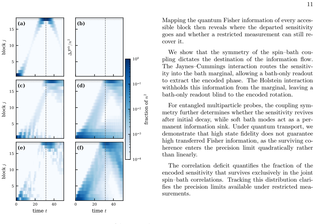
The central discovery is a destination rule: the symmetry of the spin–bath coupling alone decides which party holds the departed quantum Fisher information. For Jaynes–Cummings coupling, which conserves total excitation number, the single-excitation flow is a pure two-way exchange—F_s(j,t)=|a_j(t)|^2, F_b(j,t)=|b_j(t)|^2, and the spin–bath block adds nothing beyond its parts, so the correlation deficit vanishes identically. For Holstein coupling, which conserves spin-excitation number, the bath marginal has no term linear in the encoded angle, so a bath-only measurement returns zero first-order information; the lost sensitivity resides in spin–bath correlations, quantified by the correlation
What carries the argument
The workhorse is the block decomposition of the quantum Fisher information into spin, bath, and correlation parts, with the correlation deficit ΔF_sb = F_sb − F_s − F_b as the primary local diagnostic. For a single excitation under Jaynes–Cummings coupling, the problem reduces to independent momentum-space two-level systems with Rabi frequency Ω_q = sqrt(δ_q^2 + 4λ^2), whose occupation amplitudes are exactly the QFI densities; the bath spectrum enters through the spread of Ω_q. For Holstein coupling, a coherent boson cloud dresses each spin excitation and suppresses spin coherence by the Franck–Condon factor e^{−⟨N_b⟩}, which fixes the size of the deficit. The conserved global QFI serves as
Load-bearing premise
The claim that departed sensitivity 'never returns' assumes observations stay inside the boundary-reflection time of a finite bath; only in the infinite-chain limit is the loss strict.
What would settle it
Measure the site-summed bath QFI for a single excitation under Holstein coupling at zero encoded angle: the paper predicts exactly zero first-order information at all times, so any nonzero first-order bath QFI would falsify the destination rule. Alternatively, run a finite chain past the boundary-reflection time and watch for the predicted revival of the spin QFI, which the paper itself concedes occurs at that time.
If this is right
- For a single excitation under Jaynes–Cummings coupling, a measurement confined to the bath can recover the full phase information, since the bath QFI equals the swapped occupancy.
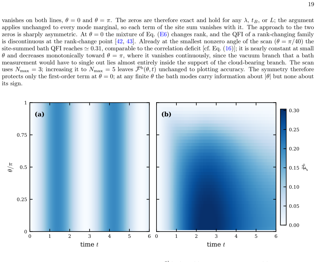
- Under Holstein coupling, a bath-only readout returns nothing to first order; recovering the lost sensitivity requires a joint spin–bath measurement, with the deficit giving the recoverable share.
- When coupled-system frequencies share a common period, departed sensitivity revives fully and periodically; when they disperse, it dephases across the bath modes and, inside the observation window, never returns.
- Soft bath modes act as a permanent information sink: as a mode frequency approaches zero, the correlation deficit climbs toward its maximum and the sensitivity it absorbs does not come back.
- A transported metrological register can arrive with high fidelity while having lost most of its usable precision, because the block QFI scales as the square of the surviving coherence, not its first power.
- For a GHZ probe on a dispersive Holstein bath, the Heisenberg advantage shrinks with probe size and can fall below the shot-noise limit, with no revival at any examined time.
Where Pith is reading between the lines
- Beyond the paper: for finite chains, 'never returns' is a windowed statement—past the boundary-reflection time the departed share would reappear; strict non-return belongs to the infinite-chain limit, so an experiment on a finite device should see recurrences on long timescales.
- Beyond the paper: metrological benchmarking of quantum channels should report Fisher information, not just transfer fidelity, since the fidelity–precision gap shown here is a generic quadratic-versus-linear effect of coherence loss.
- Beyond the paper: the Holstein first-order null is protected by parity at any temperature, but at finite nonzero probe angle the bath does register the magnitude of the rotation; a sensor could exploit this to build a coarse bath-based detector while remaining blind to the sign.
- Beyond the paper: if the destination rule extends to other generators and couplings, one could deliberately engineer a coupling symmetry to route sensitivity into a bath port as a protected memory—but only if the bath spectrum is commensurate, otherwise the information is effectively lost.
Editorial analysis
A structured set of objections, weighed in public.
Referee Report
Summary. The paper introduces a block-QFI bookkeeping decomposition for a spin chain coupled to a structured bosonic bath and asks where locally encoded phase sensitivity goes: into the bath marginal, into spin-bath correlations, or back to the spins. For a single excitation under Jaynes-Cummings coupling, the authors prove F_s(j,t)=|a_j(t)|^2, F_b(j,t)=|b_j(t)|^2, and vanishing block deficit, so the flow is a reversible two-way exchange. For Holstein coupling they prove F_b=0 at the tangent level by parity, so the lost sensitivity is carried by spin-bath correlations. They then show that the bath spectrum controls revival: commensurate frequencies return the sensitivity, dispersed frequencies dephase it. The analysis is extended to GHZ probes and to transport on engineered perfect-state-transfer chains, with closed forms for the frozen GHZ case and TEBD numerics certified in App. F. The paper is careful in distinguishing exact results from estimates, and the finite-window nature of the 'never returns' claim is stated in Sec. II and App. B.
Significance. The main conceptual contribution is a symmetry-based 'destination rule' — the form of the coupling operator decides whether a bath-only readout can recover the phase at first order — together with a spectral criterion for information return. If correct, this gives a useful diagnostic for quantum metrology beyond Lindbladian master equations. The manuscript has real strengths: the single-excitation Jaynes-Cummings sector is solved exactly (Eqs. 12 and B1-B12); the Holstein F_b=0 statement is an exact symmetry result (App. E); the frozen GHZ probe has an exact closed form for every n (Eq. 18 and App. D); and the tensor-network computations are accompanied by explicit convergence checks (Fig. 13). I also credit the authors for flagging their own limitations: App. A states precisely which steps in Eq. (16) are approximations, and Sec. II/App. B qualify the finite-chain recurrence statement. These honest caveats make the paper more trustworthy, not less. The remaining issue is presentation-level: the abstract and conclusions state the permanent-loss claim without the caveat that the body correctly supplies.
minor comments (5)
- [Abstract; Sec. VI] The abstract's 'never returns' and the concluding 'permanent information sink' are unqualified, whereas the body is careful: Sec. II says that at finite L the decay is 'effective rather than strict' because the departed share returns on the boundary-reflection time, and App. B notes that for edge encoding the reflected amplitude returns immediately, giving a few-percent to ten-percent deviation from the infinite-chain result. Since 'never' is a thermodynamic-limit extrapolation, please add a clause such as 'in the thermodynamic limit, within the pre-recurrence window' to the abstract and conclusions.
- [Sec. III B, Eq. (16)] The relation F_s≈e^{-<N_b>} is presented as a coherent-cloud estimate, and App. A correctly lists the two approximation steps and the few-percent non-coherent correction. Consider adding a one-sentence pointer to App. A directly after Eq. (16) so that a reader who does not read the appendix does not mistake the estimate for an exact identity.
- [App. B, discussion after Eq. (B7)] The discussion of the mismatch between the open chain and the infinite-chain momentum forms is important, but it appears only in the appendix. A condensed version near Fig. 3 would help, because the plotted curves there are presented as exact open-chain solutions while Eq. (B7) is the infinite-chain reference; the current placement makes the distinction easy to miss.
- [Fig. 12 caption] The caption should state explicitly that the Holstein zeros at θ=0 and θ=π are first-order zeros at the tangent level, and that the bath QFI is nonzero for intermediate θ. The main text says this, but the figure alone could be misread as saying F_b vanishes for all angles at all times.
- [Data availability] The statement 'available from the author upon reasonable request' could be replaced by a repository or DOI, especially for the TEBD datasets behind Figs. 4-8. This is a reproducibility nicety rather than a substantive requirement.
Circularity Check
No significant circularity: central QFI-flow results are derived from the Hamiltonian and exact reduced-state formulas; approximations are labeled and checked.
full rationale
The paper's main derivations are self-contained rather than circular. The conserved total QFI is fixed by the initial generator and unitarity in App. A (F_global = 4 Var(G)), independent of the coupling and not fitted to the target quantities. The Jaynes–Cummings single-excitation relations F_s(j,t)=|a_j(t)|^2, F_b(j,t)=|b_j(t)|^2, and ΔF_sb=0 follow from the exact single-particle solution (App. B) together with the reduced-state QFI formula (Eq. A8), not from assuming the result; the same holds for the bath-side derivation in App. E. The Holstein destination rule F_b=0 at θ=0 is a symmetry consequence of the density coupling being even in θ, proven in Eqs. (E5)–(E7). The approximate coherent-cloud expression 1−e^{\langle N_b\rangle} is explicitly labeled an estimate (App. A: 'both are approximations', 'a good estimate over the range computed here') and is checked against TEBD numerics, not used as a fitting input. The finite-chain "never returns" statement is explicitly qualified in Sec. II as effective rather than strict, with recurrence on the boundary-reflection time, so it is a stated approximation rather than a hidden assumption. Self-citations appear for block-QFI tools (Refs. [21–24]), but the paper re-derives the needed formulas in App. A and does not use those citations to justify its central results. No fitted parameter is renamed as a prediction, no uniqueness claim is imported from the authors' prior work, and no equation reduces to its own input by construction.
Axiom & Free-Parameter Ledger
axioms (5)
- domain assumption The joint system is closed, starts in the product state |⇑⟩|∅⟩, and evolves unitarily at zero temperature.
- domain assumption The Holstein coupling conserves spin-excitation number; the Jaynes–Cummings coupling conserves total excitation number.
- domain assumption The bath is a finite, structured reservoir; 'permanent loss' is interpreted before boundary-reflection time.
- ad hoc to paper For Eq. (16), the bath state accompanying each excitation is approximated as a coherent cloud so the overlap is e^{-nbar}.
- domain assumption For Eq. (21), the arriving block density matrix is reduced to the two-dimensional sector spanned by |↓n⟩ and |↑n⟩.
read the original abstract
We study how local sensitivity to an encoded parameter, captured by the quantum Fisher information, flows between a spin chain, a coupled bosonic bath, and their quantum correlations, where we treat the bath as a full many-body quantum system beyond the Lindbladian approximation. We analyze how the coupling symmetry determines the destination of the departed sensitivity directly at the level of the Hamiltonian. We consider an excitation-exchanging Jaynes--Cummings coupling, which preserves the total number of excitations, and a spin-excitation-conserving Holstein coupling. We find that the Holstein coupling leaves the bath with no first-order information about the phase and stores the lost sensitivity entirely in spin--bath correlations, whereas the Jaynes--Cummings coupling passes this sensitivity to the bath, in full for a single excitation. The bath spectrum then governs whether the sensitivity ever returns to the spins. It revives fully and periodically when the coupled-system frequencies share a common period, but when those frequencies disperse the departed share dephases across the bath modes and never returns. We note that a transported metrological register loses more sensitivity than its arrival fidelity implies.
Figures



Reference graph
Works this paper leans on
-
[1]
Transfer of an entan- gled multi-qubit register on such a closed chain reaches fidelities above 0.99 for up to three qubits [58]
narrives at the far end intact. Transfer of an entan- gled multi-qubit register on such a closed chain reaches fidelities above 0.99 for up to three qubits [58]. The pro- file makes the single-excitation block of the Hamiltonian the ˆJx operator of a spinj= (L−1)/2, so the single- particle propagator is a Wigner rotation matrix and the mirror time follows...
2025
-
[2]
S. L. Braunstein and C. M. Caves, Phys. Rev. Lett.72, 3439 (1994)
1994
-
[3]
M. G. A. Paris, Int. J. Quantum Inf.7, 125 (2009)
2009
-
[4]
Pezz` e, A
L. Pezz` e, A. Smerzi, M. K. Oberthaler, R. Schmied, and P. Treutlein, Rev. Mod. Phys.90, 035005 (2018)
2018
-
[5]
T´ oth and I
G. T´ oth and I. Apellaniz, J. Phys. A47, 424006 (2014)
2014
-
[6]
Giovannetti, S
V. Giovannetti, S. Lloyd, and L. Maccone, Science306, 1330 (2004)
2004
-
[7]
Giovannetti, S
V. Giovannetti, S. Lloyd, and L. Maccone, Nat. Photonics 5, 222 (2011)
2011
-
[8]
B. M. Escher, R. L. de Matos Filho, and L. Davidovich, Nat. Phys.7, 406 (2011)
2011
-
[9]
Demkowicz-Dobrza´ nski, J
R. Demkowicz-Dobrza´ nski, J. Ko lody´ nski, and M. Gut ¸˘ a, Nat. Commun.3, 1063 (2012)
2012
-
[10]
Smirne, J
A. Smirne, J. Ko lody´ nski, S. F. Huelga, and R. Demkowicz-Dobrza´ nski, Phys. Rev. Lett.116, 120801 (2016)
2016
-
[11]
Breuer and F
H.-P. Breuer and F. Petruccione,The Theory of Open Quantum Systems(Oxford University Press, 2002)
2002
-
[12]
de Vega and D
I. de Vega and D. Alonso, Rev. Mod. Phys.89, 015001 (2017)
2017
-
[13]
Breuer, E.-M
H.-P. Breuer, E.-M. Laine, and J. Piilo, Phys. Rev. Lett. 103, 210401 (2009)
2009
-
[14]
Rivas, S
´A. Rivas, S. F. Huelga, and M. B. Plenio, Phys. Rev. Lett.105, 050403 (2010)
2010
-
[15]
X.-M. Lu, X. Wang, and C. P. Sun, Phys. Rev. A82, 042103 (2010)
2010
-
[16]
A. W. Chin, S. F. Huelga, and M. B. Plenio, Phys. Rev. Lett.109, 233601 (2012)
2012
-
[17]
Rivas, S
A. Rivas, S. F. Huelga, and M. B. Plenio, Rep. Prog. Phys.77, 094001 (2014)
2014
-
[18]
Breuer, E.-M
H.-P. Breuer, E.-M. Laine, J. Piilo, and B. Vacchini, Rev. 12 Mod. Phys.88, 021002 (2016)
2016
-
[19]
Wysocki and J
P. Wysocki and J. Chwede´ nczuk, Phys. Rev. Lett.134, 020201 (2025)
2025
-
[20]
Wysocki, M
P. Wysocki, M. P lodzie´ n, and J. Chwede´ nczuk, Phys. Rev. A112, 052443 (2025)
2025
-
[21]
M. P lodzie´ n and J. Chwede´ nczuk, arXiv:2605.02774 (2026)
Pith/arXiv arXiv 2026
-
[22]
P lodzie´ n and J
M. P lodzie´ n and J. Chwede´ nczuk, Phys. Rev. Lett.136, 100204 (2026)
2026
-
[23]
Wysocki, J
P. Wysocki, J. Chwede´ nczuk, and M. P lodzie´ n, Phys. Rev. Lett.137, 030801 (2026)
2026
-
[24]
P lodzie´ n and J
M. P lodzie´ n and J. Chwede´ nczuk, Phys. Rev. A113, 062220 (2026)
2026
-
[25]
M. P lodzie´ n and J. Chwede´ nczuk, arXiv:2605.00770 (2026)
Pith/arXiv arXiv 2026
-
[26]
Holstein, Ann
T. Holstein, Ann. Phys. (N.Y.)8, 325 (1959)
1959
-
[27]
E. T. Jaynes and F. W. Cummings, Proc. IEEE51, 89 (1963)
1963
-
[28]
C. B. Duke and G. D. Mahan, Phys. Rev.139, A1965 (1965)
1965
-
[29]
G. D. Mahan,Many-Particle Physics, 3rd ed. (Kluwer Academic/Plenum, New York, 2000)
2000
-
[30]
G. M. Palma, K.-A. Suominen, and A. K. Ekert, Proc. R. Soc. Lond. A452, 567 (1996)
1996
-
[31]
T´ oth and D
G. T´ oth and D. Petz, Phys. Rev. A87, 032324 (2013)
2013
-
[32]
Gessner, L
M. Gessner, L. Pezz` e, and A. Smerzi, Phys. Rev. A94, 020101 (2016)
2016
-
[33]
W. H. Zurek, Nature Physics5, 181 (2009)
2009
-
[34]
F. G. S. L. Brand˜ ao, M. Piani, and P. Horodecki, Nature Communications6, 7908 (2015)
2015
-
[35]
Fert´ e and X
B. Fert´ e and X. Cao, Phys. Rev. Lett.132, 110201 (2024)
2024
-
[36]
Hyllus, W
P. Hyllus, W. Laskowski, R. Krischek, C. Schwemmer, W. Wieczorek, H. Weinfurter, L. Pezz´ e, and A. Smerzi, Phys. Rev. A85, 022321 (2012)
2012
-
[37]
T´ oth, Phys
G. T´ oth, Phys. Rev. A85, 022322 (2012)
2012
-
[38]
Pezz´ e and A
L. Pezz´ e and A. Smerzi, Phys. Rev. Lett.102, 100401 (2009)
2009
-
[39]
Chru´ sci´ nski and S
D. Chru´ sci´ nski and S. Maniscalco, Phys. Rev. Lett.112, 120404 (2014)
2014
-
[40]
John and J
S. John and J. Wang, Phys. Rev. Lett.64, 2418 (1990)
1990
-
[41]
Gonz´ alez-Tudela and J
A. Gonz´ alez-Tudela and J. I. Cirac, Phys. Rev. Lett.119, 143602 (2017)
2017
-
[42]
Gonz´ alez-Tudela and J
A. Gonz´ alez-Tudela and J. I. Cirac, Phys. Rev. A96, 043811 (2017)
2017
-
[43]
ˇSafr´ anek, Phys
D. ˇSafr´ anek, Phys. Rev. A95, 052320 (2017)
2017
-
[44]
Seveso, F
L. Seveso, F. Albarelli, M. G. Genoni, and M. G. A. Paris, J. Phys. A: Math. Theor.53, 02LT01 (2020)
2020
-
[45]
A. J. Leggett, S. Chakravarty, A. T. Dorsey, M. P. A. Fisher, A. Garg, and W. Zwerger, Rev. Mod. Phys.59, 1 (1987)
1987
-
[46]
W. G. Unruh, Phys. Rev. A51, 992 (1995)
1995
-
[47]
S. F. Huelga, C. Macchiavello, T. Pellizzari, A. K. Ekert, M. B. Plenio, and J. I. Cirac, Phys. Rev. Lett.79, 3865 (1997)
1997
-
[48]
Fr¨ owis and W
F. Fr¨ owis and W. D¨ ur, Phys. Rev. Lett.106, 110402 (2011)
2011
-
[49]
T. Monz, P. Schindler, J. T. Barreiro, M. Chwalla, D. Nigg, W. A. Coish, M. Harlander, W. H¨ ansel, M. Hen- nrich, and R. Blatt, Phys. Rev. Lett.106, 130506 (2011)
2011
-
[50]
J. H. Reina, L. Quiroga, and N. F. Johnson, Phys. Rev. A65, 032326 (2002)
2002
-
[51]
T. J. Proctor, P. A. Knott, and J. A. Dunningham, Phys. Rev. Lett.120, 080501 (2018)
2018
-
[52]
Zhuang, Z
Q. Zhuang, Z. Zhang, and J. H. Shapiro, Phys. Rev. A 97, 032329 (2018)
2018
-
[53]
X. Guo, C. R. Breum, J. Borregaard, S. Izumi, M. V. Larsen, T. Gehring, M. Christandl, J. S. Neergaard- Nielsen, and U. L. Andersen, Nat. Phys.16, 281 (2020)
2020
-
[54]
B. K. Malia, Y. Wu, J. Mart ´ ınez-Rinc´ on, and M. A. Ka- sevich, Nature612, 661 (2022)
2022
-
[55]
Bose, Phys
S. Bose, Phys. Rev. Lett.91, 207901 (2003)
2003
-
[56]
Christandl, N
M. Christandl, N. Datta, A. Ekert, and A. J. Landahl, Phys. Rev. Lett.92, 187902 (2004)
2004
-
[57]
Albanese, M
C. Albanese, M. Christandl, N. Datta, and A. Ekert, Phys. Rev. Lett.93, 230502 (2004)
2004
-
[58]
Kay, Int
A. Kay, Int. J. Quantum Inf.8, 641 (2010)
2010
-
[59]
Michel, M
O. Michel, M. Werner, and A. Riera, Quantum Sci. Tech- nol.11, 035006 (2026)
2026
-
[60]
Burgarth and S
D. Burgarth and S. Bose, Phys. Rev. A73, 062321 (2006)
2006
-
[61]
E. Baum, A. Broman, T. Clarke, N. C. Costa, J. Mucciac- cio, A. Yue, Y. Zhang, V. Norman, J. Patton, M. Radu- laski, and R. T. Scalettar, Phys. Rev. B105, 195429 (2022)
2022
-
[62]
Apellaniz, M
I. Apellaniz, M. Kleinmann, O. G¨ uhne, and G. T´ oth, Phys. Rev. A95, 032330 (2017). Appendix A: Reference state, block reduced states, and the block QFI Because ˆHis independent ofθ, the parameter derivative commutes with the evolution and the QFI atθ= 0 is fixed by the reference state and its tangent. Using−i ˆSy k | ↑⟩k = 1 2 | ↓⟩k, |Ψ0(t)⟩=e −i ˆHt |...
2017
-
[63]
The 2Lproblem factorizes intoLindependent two-level systems, one perq, each pairing the bare spin-excitation energyε m q =−Jcosqwith the bare boson energyε b q =ω 0 −2t B cosq
Reduction to two-level systems The swap acts on-site and conserves lattice momentumq= 2πm/L, so a spin excitation of momentumqcouples only to the boson of the same momentum. The 2Lproblem factorizes intoLindependent two-level systems, one perq, each pairing the bare spin-excitation energyε m q =−Jcosqwith the bare boson energyε b q =ω 0 −2t B cosq. Diagon...
-
[64]
The initial decay coefficient of the QFI is therefore bath-independent, fixed by the bare swap rate
Limiting regimes (i) Short times.At times short compared with every 1/Ω q, the integrand expands as sin 2(Ωqt/2)/Ω2 q =t 2/4− Ω2 qt4/48 +O(t 6), and averaging with⟨Ω 2 q⟩= 4λ 2 +ω 2 0 + 1 2 (J−2t B)2 gives ¯F s(t) = 1−λ 2t2 + λ2 12 4λ2 +ω 2 0 + 1 2 (J−2t B)2 t4 +O(t 6).(B8) The leading term−λ 2t2 is set by the coupling alone, and the bath enters only at f...
-
[65]
Perfect-transfer Hamiltonian The engineered profile breaks translation invariance, so momentum no longer labels the modes of the chain of Sec. V. The profileJ i ∝ p i(L−i) makes the single-excitation block of the Hamiltonian the ˆJx operator of a spin j= (L−1)/2,H m =−s ˆJx withs= 2J/L, so the excitation spectrum is the equally spaced ladderε m m =−s m, m...
discussion (0)
Sign in with ORCID, Apple, or X to comment. Anyone can read and Pith papers without signing in.