REVIEW 3 major objections 5 minor 44 references
This paper claims that a single closed-form spectral threshold, derived from the Weyl perturbation theorem, can purify least-squares quantum state tomography estimates and recover the true rank of photonic sensing probes without knowing it
Reviewed by Pith at T0; open to challenge. T0 means a machine referee read the full paper against a public rubric. the ladder, T0–T4 →
T0 review · deepseek-v4-flash
2026-08-01 06:35 UTC pith:Y3ODWYOT
load-bearing objection Promising but internally inconsistent rank-adaptive QST post-processor; the 20/20 rank-ID claim doesn't survive the paper's own threshold formula. the 3 major comments →
SSP-QST: Spectral Subspace Purification for Photonic Quantum State Tomography
The pith
A machine-rendered reading of the paper's core claim, the machinery that carries it, and where it could break.
Core claim
The central claim: for a least-squares estimate, the eigenvalue deficit p_hat = max(0, 1 - lambda_d) plus the shot count sets a Weyl-motivated noise floor epsilon_th = p_hat/(d-1) + 0.5/sqrt(Ns). SSP-QST eigendecomposes the estimate, keeps eigenmodes above this floor, renormalizes, and returns a purified state. Weyl's theorem bounds eigenvalue shifts by the perturbation norm; under depolarising noise on a rank-1 target, noise modes concentrate near p_hat/(d-1), so the floor separates signal from noise without a rank prior. If the second eigenvalue is below 2*epsilon_th, the method returns the dominant eigenvector; otherwise it retains all modes above the floor. The paper proves a positive fi
What carries the argument
The Weyl-motivated spectral threshold epsilon_th (Eq. 6): it turns the eigenvalue deficit p_hat = 1 - lambda_d into a noise floor by assuming depolarising noise spreads it uniformly over d-1 modes, then adds a shot-noise margin 0.5/sqrt(Ns). This threshold drives the entire algorithm: it classifies which eigenmodes survive, triggers a rank-1 override when the second eigenvalue is within 2*epsilon_th, and, after renormalization, yields a valid density matrix. The fidelity bound shows the gain scales as p(d-r)/d, which grows with dimension and shrinks as rank approaches d.
Load-bearing premise
The method trusts that the deficit 1 - lambda_d of the largest eigenvalue is entirely depolarising noise, so the computed noise floor is a true floor; if the target state itself has several comparable signal modes, that deficit contains real signal weight and the threshold can discard valid modes.
What would settle it
Take a known rank-5 or rank-6 n=4 state with near-uniform weights (e.g., Dirichlet weights near 1/r), apply depolarising noise p=0.06, simulate Ns=4096-shot LS-QST, and run SSP-QST's rank identification over many trials. If the identified rank systematically falls below the true rank at these balanced weights, while staying exact for imbalanced spectra, the noise-floor formula is confirmed to be biased by target mixing rather than by shot noise.
If this is right
- Existing least-squares QST pipelines can add SSP-QST as a drop-in layer with no change to measurement settings or shot allocation, immediately obtaining rank-adaptive purified estimates.
- For photonic probes whose effective rank exceeds 1, SSP-QST is claimed to outperform both rank-1 purification and un-purified LS-QST in reconstruction fidelity, with the largest gains over rank-1 methods at higher ranks.
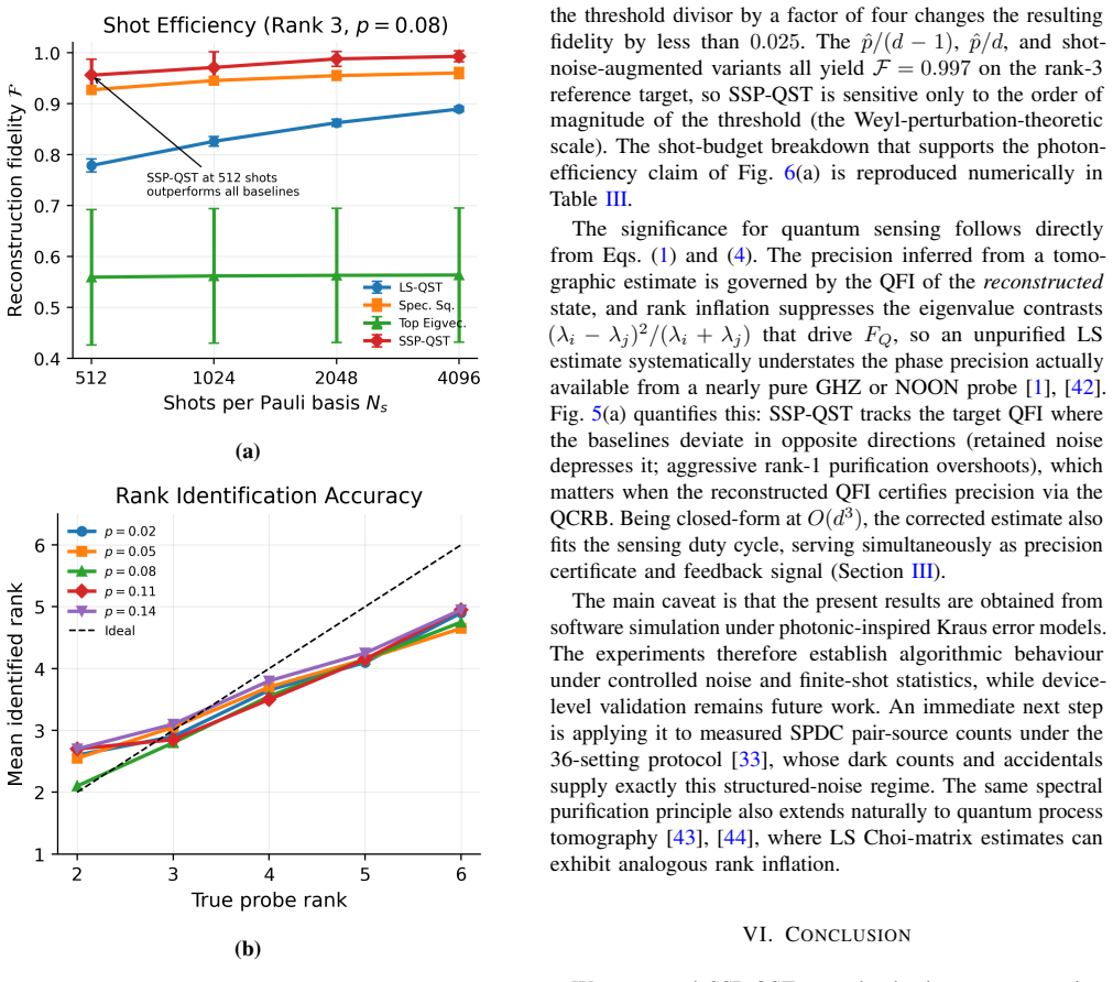
- The method reduces the shot budget needed to reach a given fidelity by at least 8x within the tested range, which matters for photon-starved sensing platforms.
- Because it is closed-form and O(d^3), the purified estimate can serve as a real-time fidelity gradient signal in feedback control loops for correcting coherent source drift.
- If the rank-identification results hold, the method provides automatic, data-driven rank selection where existing non-iterative estimators either assume rank 1 or retain full rank.
Where Pith is reading between the lines
- The threshold's noise-floor estimate assumes the dominant-eigenvalue deficit is pure depolarising noise; for genuinely mixed rank-r targets with balanced weights, the noise floor is inflated by the target's intrinsic mixing, so exact rank identification is likely to break down for higher ranks or more uniform spectra than the paper's simulated cases.
- The same spectral-purification principle should transfer to quantum process tomography, where least-squares Choi-matrix estimates suffer analogous rank inflation; the closed-form threshold would need only a re-derived noise model for the Choi representation.
- The claimed shot-efficiency and fidelity advantages are established in density-matrix simulation with analytic shot noise; device validation on real photon-counting data, such as SPDC pair sources with dark counts and accidentals, is the natural next test and could expose structured-noise regimes where the isotropic depolarising assumption is violated.
- A testable design rule follows: for fixed dimension and noise level, replacing the 0.5/sqrt(Ns) margin with a dimension-aware Bernstein bound over-truncates according to the paper's own runtime-matched comparison, so a data-driven margin calibration on real noise would settle the trade-off.
Editorial analysis
A structured set of objections, weighed in public.
Referee Report
Summary. The paper proposes SSP-QST, a closed-form post-processing layer for least-squares quantum state tomography. The method eigendecomposes the LS estimate, estimates a spectral noise floor from the largest eigenvalue and the shot count using a Weyl-perturbation-motivated threshold (Eq. 6), discards eigenvalues below this floor, and renormalizes the retained subspace, with a rank-1 override. The paper claims that this provides rank-adaptive purification without a rank prior, at O(d^3) cost, and reports Qiskit Aer simulations showing the highest fidelity among tested non-iterative baselines across probe ranks 1–7, exact rank identification for ranks 2–6 in 20/20 trials at low noise, and at least an 8× shot-efficiency improvement over LS-QST. It also gives a perturbative fidelity-gain analysis (Proposition 1 and a multi-rank extension) and a feedback controller application.
Significance. If the empirical claims were correct, SSP-QST would be a useful lightweight primitive for photonic QST and feedback-oriented sensing: the algorithm is simple, requires only one eigendecomposition, avoids iterative optimization, and the paper is honest that Eq. (6) is exact only for depolarizing noise and that experiments are simulations. The algebraic derivation of Proposition 1 is internally consistent under its stated alignment and eigengap assumptions. However, the central rank-adaptivity claim is undermined by an apparent internal inconsistency: under the paper's own flat-Dirichlet target-weight model, the threshold in Eq. (6) interprets the dominant-eigenvalue deficit as noise, so it can discard genuine small signal modes for ranks 5–6. This directly contradicts the reported 20/20 exact rank identification and the advertised 'no rank prior' capability, and needs to be resolved before the results can be accepted.
major comments (3)
- [Eq. (6), §IV-A/IV-F, Table II] The reported 20/20 exact rank identification for r=5,6 is inconsistent with the stated model. Under flat Dir(1,...,1) weights, λ_d ≈ w_max, so p̂ ≈ 1 − w_max + p(w_max − 1/d); the first term of ε_th is (1−w_max)/(d−1), which is target mixing, not noise. For r=6, E[w_max]=H_6/6≈0.408 and E[w_min]=1/36≈0.0278; at p=0.06, Ns=4096, ε_th≈0.049 while the smallest true signal eigenvalue is (1−p)w_min+p/d≈0.030. Thus the smallest mode lies below the threshold for typical draws, so exact rank identification cannot hold in 20/20 trials. Table II's F=0.965 at r=6 is consistent with dropping the smallest mode (1−E[w_min]≈0.972). Please provide the actual target weights/code or correct the claim.
- [§III-C, multi-rank extension] The multi-rank fidelity analysis assumes the eigengap λ^tgt_r > ε_th + ||Δ||_2 and alignment as hypotheses; it therefore does not by itself establish that SSP-QST recovers the rank. In the simulated Dirichlet model this condition is violated for the smallest modes at r=5–6, so the theoretical analysis does not cover the regime where the paper claims exact identification. The statement that underestimating the rank is the 'safe' failure mode (Section III-A, IV-F) is also misleading: dropping a true small signal mode is exactly the rank-one failure mode the paper motivates against. Please provide a rank-selection failure-probability bound or verify the eigengap condition empirically for each reported setting.
- [§IV-H, runtime-matched ML comparison] The runtime-matched comparison in Section IV-H compares SSP-QST against a single RρR iteration from the maximally mixed seed and reports very low ML fidelities (0.07–0.37). This is not a meaningful measure of ML's reconstruction capability; it only shows that one iteration is insufficient. The generous-budget comparison is more informative, but the conclusion that unregularised ML retains a noise pedestal is really a property of the estimator and the measurement model, not of the runtime budget. This section should be reframed as a latency-constrained comparison, not as evidence against iterative ML in general.
minor comments (5)
- [§IV-A vs Fig. 3 caption] The number of random targets is inconsistent: §IV-A says '8 to 10', Fig. 3 says '14 independently drawn', §IV-F says '20 trials'. Please harmonize.
- [Eq. (6)] The shot-noise term is written as '0.5√Ns'; from the text it should be '0.5/√Ns'. Please fix the typography to avoid ambiguity.
- [Table IV] The first threshold variant (p̂/(2d)+0.5/√Ns) identifies rank 4, not 3. The claim that 'the identified rank remains correct for the default and nearby settings' should be qualified, and the 'safe' direction is under-estimation, whereas this variant over-estimates.
- [§V, Discussion] The phrase 'depolarised mixtures sit closer to higher-rank targets under fidelity' is grammatically incomplete; suggest 'under the fidelity measure'.
- [General] A code/data availability statement would greatly help reproducibility, especially for the 20/20 rank-identification claim and the exact target-weight draws.
Circularity Check
No substantive circularity: the spectral threshold is data-calibrated and the central fidelity/rank-ID claims are independent simulation results; the only self-citation is peripheral.
full rationale
The core derivation is not circular. Eq. (6) sets epsilon_th from p_hat = max(0, 1 - lambda_d) and the shot count; the reconstructed rank is the number of eigenvalues exceeding this floor, so the method's output rank is not fed back into the definition of the floor (Section III-A, Algorithm 1). This is a self-calibrating estimator, not a quantity defined in terms of the predicted rank. The fidelity-gain bound (Prop. 1, Eq. 7) is a direct Uhlmann-fidelity computation under the stated pure-target, alignment, and eigengap assumptions; the gains in Table II/Fig. 3 are evaluated against independently drawn random targets, so they are not forced by the threshold formula. The rank-r extension (Eqs. 10-11) uses an explicit eigengap condition and is not a restatement of the input. The only self-citation, [19] by co-author Mukhopadhyay, supports FPGA feasibility together with independent [20]; it is not load-bearing for the rank-adaptivity or fidelity claims. The paper itself flags the scope limitation: 'Under amplitude damping or phase damping... Eq. (6) is a heuristic motivated by the Weyl scale rather than a rigorously derived bound,' and the main caveat that results are software simulations. The reported 20/20 exact rank-ID for ranks 5-6 is in numerical tension with Eq. (6) for flat Dirichlet weights, but that is an internal-consistency/correctness risk, not a circular reduction, so it does not raise the circularity score.
Axiom & Free-Parameter Ledger
free parameters (3)
- shot-noise margin coefficient =
0.5 (in 0.5/sqrt(N_s))
- noise-floor divisor =
d-1 (in p_hat/(d-1))
- rank-1 override factor =
2 (lambda_{d-1} < 2*epsilon_th)
axioms (6)
- domain assumption Eigenvalues of the depolarized target concentrate: true signal eigenvalues ~ (1-p)w_i + p/d, noise eigenvalues ~ p/d.
- standard math Shot-noise eigenvalue fluctuations delta_lambda_i are sub-Gaussian with Var <= 1/(dN_s), via first-order perturbation theory and Pauli completeness.
- standard math Weyl bound |lambda_i(rho_LS)-lambda_i(rho_tgt)| <= ||Delta||_2 and matrix-Bernstein bound ||Delta_shot||_2 <= sqrt(2 ln(2d)/N_s).
- ad hoc to paper Alignment conditions |<v_d|psi>| ~ 1 (rank-1) and |<v_{d-j+1}|phi_j>| ~ 1 (rank-r), plus eigengap lambda^tgt_r > epsilon_th + ||Delta||_2.
- domain assumption Qiskit Aer density-matrix backend exactly implements Kraus evolution and the shot statistics of Eq. (2); simulation stands in for experiment.
- domain assumption Rank-r probes are orthonormal mixtures sum w_i|phi_i><phi_i| with w ~ Dir(1,...,1) and Haar-distributed frames from QR of a Ginibre matrix.
read the original abstract
Photonic quantum sensing often uses low-rank entangled probes such as Greenberger-Horne-Zeilinger (GHZ), Bell, and NOON states. Although these probes are ideally rank-1, practical quantum state tomography (QST) can produce density-matrix estimates with many small finite-shot and noise-induced eigenmodes. This eigenvalue contamination can increase the estimated entropy of the reconstruction and reduce the quantum Fisher information (QFI) available for downstream sensing, while fixed rank-1 purification can discard valid signal modes when real probes acquire additional signal modes. We introduce Spectral Subspace Purification for Quantum State Tomography (SSP-QST), a rank-adaptive post-processing layer for least-squares quantum state tomography (LS-QST). SSP-QST eigendecomposes the least-squares estimate, computes a Weyl-motivated noise floor from the measured spectrum and shot count, removes eigenmodes below this floor, and renormalises the retained subspace. It requires no rank prior, no iterative optimisation, and only one eigendecomposition. In Qiskit Aer simulations, SSP-QST achieves the highest fidelity among the tested non-iterative baselines across the evaluated probe ranks, with a maximum fidelity gain of $+0.584$. It also improves shot efficiency by at least $8\times$ within the tested range. These results show that SSP-QST can make photonic QST more reliable under finite-shot noise while providing a lightweight reconstruction primitive for feedback-oriented quantum sensing pipelines.
Figures


Reference graph
Works this paper leans on
-
[1]
Quantum-enhanced measure- ments: Beating the standard quantum limit,
V . Giovannetti, S. Lloyd, and L. Maccone, “Quantum-enhanced measure- ments: Beating the standard quantum limit,”Science, vol. 306, no. 5700, pp. 1330–1336, 2004
2004
-
[2]
Photonic quantum information pro- cessing: A concise review,
S. Slussarenko and G. J. Pryde, “Photonic quantum information pro- cessing: A concise review,”Applied Physics Reviews, vol. 6, no. 4, p. 041303, 2019
2019
-
[3]
Quantum fisher information matrix and multiparameter estimation,
J. Liu, H. Yuan, X.-M. Lu, and X. Wang, “Quantum fisher information matrix and multiparameter estimation,”Journal of Physics A: Mathemat- ical and Theoretical, vol. 53, no. 2, p. 023001, 2020
2020
-
[4]
Quantum computational advantage with a pro- grammable photonic processor,
L. S. Madsenet al., “Quantum computational advantage with a pro- grammable photonic processor,”Nature, vol. 606, pp. 75–81, 2022
2022
-
[5]
Multipartite entanglement and high-precision metrology,
G. Tóth and I. Apellaniz, “Multipartite entanglement and high-precision metrology,”Physical Review A, vol. 85, no. 2, p. 022322, 2012
2012
-
[6]
Photonic state tomography,
J. B. Altepeter, E. R. Jeffrey, and P. G. Kwiat, “Photonic state tomography,” Advances in Atomic, Molecular, and Optical Physics, vol. 52, pp. 105– 159, 2005
2005
-
[7]
Quantum limits in optical interferometry,
R. Demkowicz-Dobrza ´nski, M. Jarzyna, and J. Kołody ´nski, “Quantum limits in optical interferometry,”Progress in Optics, vol. 60, pp. 345–435, 2015
2015
-
[8]
Efficient quantum state tomography,
M. Cramer, M. B. Plenio, S. T. Flammia, R. Somma, D. Gross, S. D. Bartlett, O. Landon-Cardinal, D. Poulin, and Y .-K. Liu, “Efficient quantum state tomography,”Nature Communications, vol. 1, no. 1, p. 149, 2010
2010
-
[9]
Quantum state tomography via compressed sensing,
D. Gross, Y .-K. Liu, S. T. Flammia, S. Becker, and J. Eisert, “Quantum state tomography via compressed sensing,”Physical Review Letters, vol. 105, no. 15, p. 150401, 2010
2010
-
[10]
Quantum-state estimation,
Z. Hradil, “Quantum-state estimation,”Physical Review A, vol. 55, no. 3, p. R1561, 1997
1997
-
[11]
Diluted maximum- likelihood algorithm for quantum tomography,
J. ˇReháˇcek, Z. Hradil, E. Knill, and A. I. Lvovsky, “Diluted maximum- likelihood algorithm for quantum tomography,”Physical Review A, vol. 75, no. 4, p. 042108, 2007
2007
-
[12]
Fast and noise-robust quantum state tomography based on ELM,
X.-D. Wu and S. Cong, “Fast and noise-robust quantum state tomography based on ELM,”International Journal of Quantum Information, vol. 22, no. 04, p. 2350052, 2024
2024
-
[13]
Hedged maximum likelihood quantum state estima- tion,
R. Blume-Kohout, “Hedged maximum likelihood quantum state estima- tion,”Physical Review Letters, vol. 105, no. 20, p. 200504, 2010
2010
-
[14]
Quantum state tomography via linear regression estimation,
B. Qi, Z. Hou, L. Li, D. Dong, G. Xiang, and G. Guo, “Quantum state tomography via linear regression estimation,”Scientific Reports, vol. 3, p. 3496, 2013
2013
-
[15]
Adaptive quantum state tomography via linear regression estimation: Theory and two-qubit experiment,
B. Qi, Z. Hou, Y . Wang, D. Dong, H.-S. Zhong, L. Li, G.-Y . Xiang, H. M. Wiseman, C.-F. Li, and G.-C. Guo, “Adaptive quantum state tomography via linear regression estimation: Theory and two-qubit experiment,”npj Quantum Information, vol. 3, no. 1, p. 19, 2017
2017
-
[16]
Efficient learning algorithms for noisy quantum state and process tomography,
C. Li, S. Zhuang, Y . Zhang, J. B. Wang, X. Yuan, Y . Wu, and C. Wang, “Efficient learning algorithms for noisy quantum state and process tomography,”arXiv preprint arXiv:2603.01521, 2026
Pith/arXiv arXiv 2026
-
[17]
Robust quantum state tomography method for quantum sensing,
A. Farooq, U. Khalid, J. u. Rehman, and H. Shin, “Robust quantum state tomography method for quantum sensing,”Sensors, vol. 22, no. 7, p. 2669, 2022
2022
-
[18]
Experimental ver- ification of threshold quantum state tomography on a fully-reconfigurable photonic integrated circuit,
E. Caruccio, D. Maragnano, G. Rodari, D. Picus, G. Garberoglio, D. Bi- nosi, R. Albiero, N. Di Giano, F. Ceccarelli, G. Corrielli, N. Spagnolo, R. Osellame, M. Dapor, M. Liscidini, and F. Sciarrino, “Experimental ver- ification of threshold quantum state tomography on a fully-reconfigurable photonic integrated circuit,”npj Quantum Information, vol. 11, p....
2025
-
[19]
A reconfigurable quantum state tomography solver in FPGA,
N. E. Miller, B. Chakraborty, and S. Mukhopadhyay, “A reconfigurable quantum state tomography solver in FPGA,” in2023 IEEE International Conference on Quantum Computing and Engineering (QCE). IEEE, 2023, pp. 1412–1421
2023
-
[20]
Machine learning enhanced quantum state tomography on a field-programmable gate array,
H.-C. Wu, H.-Y . Hsieh, Z.-K. Xu, H. L. Chen, Z.-H. Shi, P.-H. Wang, P. Yang, O. Steuernagel, T.-H. Suen, C.-M. Wu, and R.-K. Lee, “Machine learning enhanced quantum state tomography on a field-programmable gate array,”APL Quantum, vol. 2, no. 2, p. 026117, 2025
2025
-
[21]
Paris and J
M. Paris and J. ˇReháˇcek, Eds.,Quantum State Estimation, ser. Lecture Notes in Physics. Springer, 2004, vol. 649
2004
-
[22]
Efficient method for computing the maximum-likelihood quantum state from measurements with additive gaussian noise,
J. A. Smolin, J. M. Gambetta, and G. Smith, “Efficient method for computing the maximum-likelihood quantum state from measurements with additive gaussian noise,”Physical Review Letters, vol. 108, no. 7, p. 070502, 2012
2012
-
[23]
Quantum tomography via compressed sensing: error bounds, sample complexity and efficient estimators,
S. T. Flammia, D. Gross, Y .-K. Liu, and J. Eisert, “Quantum tomography via compressed sensing: error bounds, sample complexity and efficient estimators,”New Journal of Physics, vol. 14, no. 9, p. 095022, 2012
2012
-
[24]
Fast state tomography with optimal error bounds,
M. Gu¸ t˘a, J. Kahn, R. Kueng, and J. A. Tropp, “Fast state tomography with optimal error bounds,”Journal of Physics A: Mathematical and Theoretical, vol. 53, no. 20, p. 204001, 2020
2020
-
[25]
Projected least- squares quantum process tomography,
T. Surawy-Stepney, J. Kahn, R. Kueng, and M. Gu¸ t˘a, “Projected least- squares quantum process tomography,”Quantum, vol. 6, p. 844, 2022
2022
-
[26]
Streaming quantum state purification,
A. M. Childs, H. Fu, D. Leung, Z. Li, M. Ozols, and V . Vyas, “Streaming quantum state purification,”Quantum, vol. 9, p. 1603, 2025
2025
-
[27]
Optimal, reliable estimation of quantum states,
R. Blume-Kohout, “Optimal, reliable estimation of quantum states,”New Journal of Physics, vol. 12, p. 043034, 2010
2010
-
[28]
Neural-network quantum state tomography,
G. Torlai, G. Mazzola, J. Carrasquilla, M. Troyer, R. Melko, and G. Carleo, “Neural-network quantum state tomography,”Nature Physics, vol. 14, no. 5, pp. 447–450, 2018
2018
-
[29]
Maximum likelihood quantum state tomography is inadmissible,
C. Ferrie and R. Blume-Kohout, “Maximum likelihood quantum state tomography is inadmissible,”arXiv preprint arXiv:1808.01072, 2018
Pith/arXiv arXiv 2018
-
[30]
Robustness analysis in static and dynamic quantum state tomography,
A. Chen, S. Xiao, H. Ma, and D. Dong, “Robustness analysis in static and dynamic quantum state tomography,”arXiv preprint arXiv:2512.12518, 2025
arXiv 2025
-
[31]
Perturbative quantum-state estimation,
P. Banáš, J. ˇReháˇcek, and Z. Hradil, “Perturbative quantum-state estimation,”Physical Review A, vol. 74, p. 014101, 2006
2006
-
[32]
Maximum-likelihood estimation of the density matrix,
K. Banaszek, G. M. D’Ariano, M. G. A. Paris, and M. F. Sacchi, “Maximum-likelihood estimation of the density matrix,”Physical Review A, vol. 61, p. 010304, 1999
1999
-
[33]
Measurement of qubits,
D. F. V . James, P. G. Kwiat, W. J. Munro, and A. G. White, “Measurement of qubits,”Physical Review A, vol. 64, p. 052312, 2001
2001
-
[34]
Continuous-variable optical quantum- state tomography,
A. I. Lvovsky and M. G. Raymer, “Continuous-variable optical quantum- state tomography,”Reviews of Modern Physics, vol. 81, pp. 299–332, 2009
2009
-
[35]
Spectral thresholding quantum tomography for low rank states,
C. Butucea, M. Gu¸ t˘a, and T. Kypraios, “Spectral thresholding quantum tomography for low rank states,”New Journal of Physics, vol. 17, p. 113050, 2015
2015
-
[36]
A comparative study of estimation methods in quantum tomography,
A. Acharya, T. Kypraios, and M. Gu¸ t˘a, “A comparative study of estimation methods in quantum tomography,”Journal of Physics A: Mathematical and Theoretical, vol. 52, no. 23, p. 234001, 2019
2019
-
[37]
Bhatia,Matrix Analysis
R. Bhatia,Matrix Analysis. Springer, 1997
1997
-
[38]
An introduction to matrix concentration inequalities,
J. A. Tropp, “An introduction to matrix concentration inequalities,” Foundations and Trends in Machine Learning, vol. 8, no. 1–2, pp. 1–230, 2015
2015
-
[39]
The transition probability in the state space of a ∗-algebra,
A. Uhlmann, “The transition probability in the state space of a ∗-algebra,” Reports on Mathematical Physics, vol. 9, no. 2, pp. 273–279, 1976
1976
-
[40]
Qiskit: An open-source sdk for quantum computing,
Qiskit contributors, “Qiskit: An open-source sdk for quantum computing,” https://pypi.org/project/qiskit/, 2026, version 2.4.1, accessed 2026-04-28
2026
-
[41]
Probabilistic error cancellation with sparse pauli–lindblad models on noisy quantum processors,
E. van den Berg, Z. K. Minev, A. Kandala, and K. Temme, “Probabilistic error cancellation with sparse pauli–lindblad models on noisy quantum processors,”Nature Physics, vol. 19, pp. 1116–1121, 2023
2023
-
[42]
Quantum sensing,
C. L. Degen, F. Reinhard, and P. Cappellaro, “Quantum sensing,”Reviews of Modern Physics, vol. 89, p. 035002, 2017
2017
-
[43]
Quantum circuit architecture,
G. Chiribella, G. M. D’Ariano, and P. Perinotti, “Quantum circuit architecture,”Physical Review Letters, vol. 101, no. 6, p. 060401, 2008
2008
-
[44]
M. Dinca, D. J. Luitz, and M. Debertolis, “Quantum process tomography of a compressed time evolution circuit on superconducting quantum processors,”arXiv preprint arXiv:2509.25342, 2025
arXiv 2025
discussion (0)
Sign in with ORCID, Apple, or X to comment. Anyone can read and Pith papers without signing in.