REVIEW 2 major objections 5 minor 22 references
Two outcomes that push on each other within the same measurement window usually defeat causal analysis without instruments; this paper proves that feature-dependent variation in the two structural shock variances is enough to separate the t
Reviewed by Pith at T0; open to challenge. T0 means a machine referee read the full paper against a public rubric. the ladder, T0–T4 →
T0 review · deepseek-v4-flash
2026-08-01 05:08 UTC pith:VWE64HRQ
load-bearing objection Solid population identification theory and an honest Monte Carlo, but the neural-transfer assumption (N2) is effectively the conclusion of the theorem, and the finite-sample bias for gamma1 is large; deserves review but not unqualified acceptance. the 2 major comments →
Learning Bidirectional Causal Interactions with Heteroscedastic Neural Networks
The pith
A machine-rendered reading of the paper's core claim, the machinery that carries it, and where it could break.
Core claim
In the paper's own terms, the discovery is an identification result with an explicit curvature computation. For any candidate γ, the mean-profiled residuals satisfy r_γ = Γ(γ)Γ0⁻¹ ε, so a misspecified γ mixes the two structural shocks and induces conditional correlation between the residual components. The unrestricted profiled quasi-likelihood Q*(γ) is shown to expand as Q*(γ0 + h) − Q*(γ0) = −(1/2) hᵀ I*_γ h + o(‖h‖²) with I*_γ = (1/d0²)[[E{ρ0(x)⁻¹}, 1], [1, E{ρ0(x)}]], where ρ0(x) = g10(x)/g20(x) is the variance ratio. Since E{ρ}E{ρ⁻¹} > 1 exactly when ρ0 is not almost surely constant, I*_γ is positive definite, making γ0 a strict local maximizer; a companion lemma shows γ0 is the unique
What carries the argument
The carrying object is the diagonalization identity at the center of the argument: the residual covariance under a candidate interaction vector is Vγ(x) = Γ(γ)Γ0⁻¹ diag(g10(x), g20(x)) (Γ(γ)Γ0⁻¹)ᵀ, whose off-diagonal term is nonzero for any γ ≠ γ0 unless the variance ratio ρ0(x) is constant. Around this sit the components that make the argument work: the diagonal Gaussian quasi-likelihood with the simultaneous-system Jacobian log|det Γ(γ)|; the profiled curvature matrix I*_γ whose off-diagonal entries are identically 1; the Cauchy–Schwarz step E{ρ}E{ρ⁻¹} ≥ 1 with equality iff ρ0 is constant; and the quotient-slice construction that treats network weights inducing the same functions as equiva
Load-bearing premise
Everything falls apart unless the variance ratio ρ0(x) = g10(x)/g20(x) genuinely varies over the feature space and the neural networks can locally reproduce the profiled conditional mean and variance functions to second order — the load-bearing step is the neural-profile compatibility condition (Assumption 3(N2)), which the paper does not verify constructively.
What would settle it
Generate data from the paper's own design but replace g2(x) with an exact copy of g1(x), making the variance ratio constant while keeping everything else identical; the theory predicts a flat direction in the profile, so estimates of γ1 and γ2 cannot both converge. The direct check is numeric: compute the sample analogue of I*_γ and look at det(Ĥρ) = mean(ρ) mean(ρ⁻¹) − 1, which should be near zero in that design and clearly positive in designs where identification is claimed to hold.
If this is right
- Two-way contemporaneous effects are identifiable from conditional second moments alone; external instruments are not required when the shock variances vary non-proportionally.
- The variance networks in SEM-DNN do identification work, not just uncertainty calibration; the fitted variance-ratio matrix tells the analyst whether identification is strong or near-empty, with determinant zero exactly when the fitted variance ratio is constant.
- Separate flexible regressions systematically confuse structural feedback with reduced-form dependence, and the simulation evidence indicates that bias does not vanish with sample size; only a system-level likelihood with the Jacobian distinguishes the two directions.
- The causal reading of the recovered coefficients holds exactly when the equations are interpreted as autonomous, intervention-invariant mechanisms; statistical identification alone does not supply causality.
- Held-out diagnostics — residual-diagonalization moments, variance calibration, and gradient leverage — give concrete checks on whether the identifying assumptions are plausible for a given dataset.
Where Pith is reading between the lines
- If the identification result is right, the same curvature formula suggests an immediate extension to feedback systems with more than two outcomes: the scalar ratio ρ0 would be replaced by the ratio matrix of shock variances, and identification would require the joint distribution of those ratios to be non-degenerate — a testable simulation design.
- A practical consequence of the theorem is that every fitted model should report the sample analogue of I*_γ; when the empirical distribution of the fitted variance ratio is tight, the profiled criterion is nearly flat, and seed-to-seed dispersion in the interaction estimates becomes a warning sign of weak identification rather than a numerical artifact.
- The paper's empirical application leaves the causal reading deliberately qualified; a natural follow-up is to add historical instruments or exclusion restrictions and test whether the heteroscedasticity-based estimates move, which would probe the conditional-shock-orthogonality assumption that diagnostics can only partially check.
Editorial analysis
A structured set of objections, weighed in public.
Referee Report
Summary. The paper proposes SEM-DNN, a heteroscedastic neural estimator for a two-equation simultaneous system y1 = γ1 y2 + f1(x) + ε1, y2 = γ2 y1 + f2(x) + ε2, where f1, f2, and the conditional variances g1, g2 are unknown nonlinear functions represented by neural networks. Identification of the interaction coefficients (γ1, γ2) is based on conditional covariance diagonalization: under zero conditional mean, conditional uncorrelatedness of the shocks given x, and a nonconstant conditional variance ratio ρ0(x) = g10(x)/g20(x), only the true γ makes the transformed residuals conditionally uncorrelated across the feature space. The paper derives a profiled population criterion Q*(γ), proves a local second-order curvature result (Proposition 1), a global diagonalization uniqueness result (Lemma 1), and a local neural identification theorem (Theorem 1) under an explicit neural-profile compatibility condition. A stabilized training objective with β-NLL weighting and bounded γ-parameterization is introduced, followed by Monte Carlo experiments and a Dominick's scanner-data application with extensive diagnostics. The paper is careful to separate causal-interpretation assumptions from statistical identification assumptions and to present the empirical illustration as a workflow demonstration rather than a definitive estimate.
Significance. If the identification result is accepted, the paper makes a useful contribution: it shows that conditional heteroscedasticity can identify two contemporaneous structural interaction coefficients without external instruments, while allowing flexible neural nuisance functions. Proposition 1 and Lemma 1 are cleanly derived: the covariance expansion is algebraically correct, and the Cauchy-Schwarz argument for positive definiteness of I*γ is sound. The paper also ships an unusually transparent empirical protocol, including sample-construction timing rules, held-out diagnostics, seedwise reporting, and detailed Monte Carlo and robustness descriptions. The main risk is that Theorem 1's transfer from the population profiled criterion to the neural-profile criterion is largely assumed rather than derived; the strength of the paper's central claim therefore rests on an assumption that is not constructively verified.
major comments (2)
- [Assumption 3(N2), §2.2] The central transfer from the unrestricted profiled criterion to the neural profile is assumed, not derived. Assumption 3(N2) requires, for every h near zero, a path a*(h) such that the neural mean and variance networks represent the unrestricted profiled functions m*γ,k and v*γ,k up to o(||h||^2) error, equivalently Qδ,η0(γ0+h) = Q*(γ0+h) + o(||h||^2). This is precisely the inheritance property needed for Theorem 1. No primitive conditions on network width/depth, activation class, or DGP smoothness are supplied from which such a path follows; universal approximation of a fixed function does not imply second-order approximation of a γ-indexed family of conditional expectations. If N2 fails, the implemented criterion's curvature is the Schur complement Jγγ − Jγη Jηη+ Jηγ, which need not equal I*γ, and local identification could be weak or absent. The paper states N2 as an assumption, so T
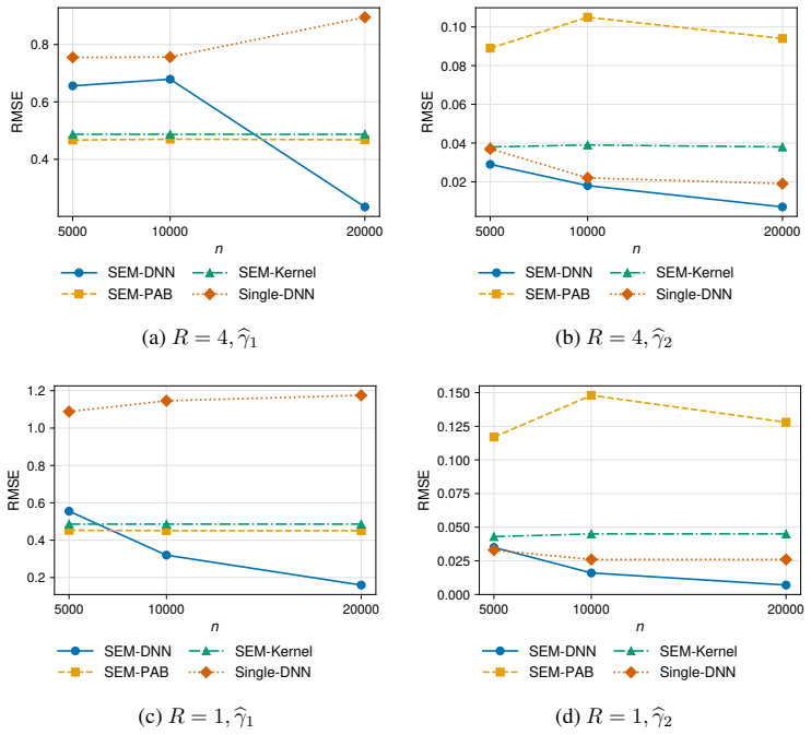
- [Table D.1 and Section D.1] Section D.1 states that c=0 recovers the baseline variance design. For n=10,000 and R=4, Table D.1 reports mean bias −0.478 and RMSE 0.679 for γ1. If c=0 is indeed the baseline, this is a very large bias relative to the true γ1=0.5 and appears inconsistent with the visual impression of the main Monte Carlo figures; if the D.1 protocol differs from the main design, the text should say so explicitly. More generally, at n=10,000 the estimator is far from unbiased, and without a consistency theorem the claim that SEM-DNN 'recovers structural effects more reliably as information increases' rests heavily on the n=20,000 results. The authors should reconcile this table with the main Monte Carlo presentation and either provide the n=20,000 analogue for the D.1 design or qualify the empirical claim.
minor comments (5)
- [General notation] Several key equations, including the definition of I*γ in §2.3, are not numbered; numbering would make the paper easier to referee and reuse.
- [§3.2] The β-NLL weight uses si(α1,α2) and ¯sB(α1,α2); it would help to state explicitly that the stop-gradient operator applies only to the weight, not to qi(θ), since the text is otherwise easy to misread.
- [§5.2] The seedwise interquartile ranges are described as not confidence intervals, which is appropriate. The representative-seed choice ('lower median rank') is explained in the appendix; a one-sentence reminder in the main text would improve readability.
- [Appendix D.1] The column label 'Param' in Table D.1 is cryptic; using 'Coefficient' or 'Parameter' would be clearer.
- [Appendix E] The sample-construction protocol is very detailed and transparent; consider adding a short statement on code/data availability for the replication pipeline, since the text repeatedly refers to 'replication output' without giving a location.
Circularity Check
The neural curvature-transfer theorem restates Assumption 3(N2): the conclusion that the neural profile inherits I*γ is exactly the compatibility assumption plus Proposition 1.
specific steps
-
self definitional
[Section 2.2, Assumption 3(N2); Section 2.3, Theorem 1; Appendix A.3]
"Assumption 3 (N2): ... Equivalently, Qδ,η0(γ0 + h) = Q∗(γ0 + h) + o(∥h∥2), h → 0. ... Theorem 1: Qδ,η0(γ0 +h)−Qδ,η0(γ0) = − 1 2 h⊤I∗γ h+o(∥h∥2). Proof: 'By Assumption 3 (N2), the local neural profiled criterion satisfies Qδ,η0(γ0 +h) = Q∗(γ0 +h) + o(∥h∥2).'"
Theorem 1's displayed expansion is obtained by substituting Proposition 1 into Assumption 3(N2). N2 already asserts that the neural profiled criterion equals the unrestricted profile to o(||h||^2); Proposition 1 then supplies the quadratic term -1/2 h^T I*γ h. Therefore the central claim that the implemented neural criterion inherits the population curvature is not derived from primitive network or DGP conditions—it is assumed verbatim as the compatibility condition. Appendix A.3's proof says 'By Assumption 3 (N2)...' and then combines it with Proposition 1, so the neural-curvature result is the input itself. No width/depth/activation/smoothness argument establishes the existence of a*(h).
full rationale
The population-level identification argument is self-contained: Proposition 1 and Lemma 1 derive the profiled curvature and unique diagonalization directly from Assumption 2 via a second-order expansion of the unrestricted profiled quasi-likelihood, without using fitted neural outputs as targets. The one self-citation ([16]) is an extension of the same heteroscedasticity approach and is not load-bearing. However, the neural-transfer step is circular in a narrow but important sense: Assumption 3(N2) is defined as the statement that the local neural profile matches Q* to o(||h||^2), and Theorem 1's conclusion (curvature I*γ and local identification on the quotient slice) is exactly that assumption combined with Proposition 1. The paper is transparent that Assumption 3 is a compatibility condition rather than a primitive source of identification, so the Q* identification retains independent content; but the headline claim that the implemented criterion 'inherits' the curvature is, by the paper's own equations, an assumption rather than a derivation. Finite-sample bias in the Monte Carlo baseline is a correctness risk, not additional circularity. Overall: partial circularity in the neural inheritance theorem, independent population identification.
Axiom & Free-Parameter Ledger
free parameters (5)
- g_min =
0.01
- β (β-NLL stabilization) =
0.5
- ¯γ (stability bound) =
0.99
- Regularization vector φ =
Selected by Sobol/validation over log10 penalties in [-8,-1]
- Network architecture =
2 hidden layers × 256 units, GELU, per network
axioms (6)
- domain assumption Assumption 2(S2): E(ε|x)=0 and Var(ε|x)=diag(g10(x),g20(x))
- domain assumption Assumption 2(S3): 0<cρ≤ρ0(x)=g10/g20≤Cρ<∞ and ρ0 is not almost surely constant
- domain assumption Assumption 1: structural equations are autonomous and invariant under the relevant interventions
- ad hoc to paper Assumption 3(N1–N3): neural-profile compatibility, local paths representing unrestricted profiled functions, and Hessian kernel inclusion ker(Jηη)⊆ker(Jγη)
- domain assumption Stable parameter region |γk|≤¯γ<1
- standard math Standard analytic tools: dominated convergence, Cauchy-Schwarz, Schur complement
read the original abstract
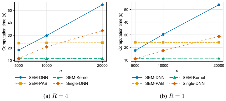
Estimating contemporaneous bidirectional interactions from observational data is difficult because each outcome is endogenous to the other, while flexible regressions may capture only reduced-form dependence. This paper proposes SEM-DNN, a heteroscedastic neural simultaneous-equation estimator that learns reciprocal structural interactions without external instruments. Identification exploits conditional covariance diagonalization: when structural shocks have zero conditional means, are conditionally uncorrelated given predetermined covariates, and exhibit nonproportional conditional variances, only the true interaction coefficients diagonalize the conditional residual covariance across the feature space. The method jointly approximates nonlinear structural mean functions and feature-dependent variances using a diagonal Gaussian quasi-likelihood that incorporates the simultaneous-system Jacobian. We establish unique identification and positive-definite local curvature of the profiled population criterion and show that, under neural-profile compatibility conditions, the implemented neural criterion inherits this curvature despite nonunique network parameterizations. The coefficients admit a causal interpretation when the structural equations represent autonomous mechanisms that remain invariant under the relevant interventions. Monte Carlo experiments with nonlinear, high-dimensional nuisance functions and non-Gaussian shocks show that SEM-DNN recovers structural effects more reliably than parametric, kernel-based, and separate-equation neural alternatives as information increases, although at greater computational cost. An application to ready-to-eat cereal scanner data illustrates how the method can study contemporaneous price-sales feedback and assess identification strength, residual diagonalization, variance calibration, and optimization sensitivity.
Figures




Reference graph
Works this paper leans on
-
[1]
Causal machine learning for predicting treatment outcomes , year =
Feuerriegel, Stefan and Frauen, Dennis and Melnychuk, Valentyn and Schweisthal, Jonas and Hess, Konstantin and Curth, Alicia and Bauer, Stefan and Kilbertus, Niki and Kohane, Isaac S and van der Schaar, Mihaela , journal =. Causal machine learning for predicting treatment outcomes , year =
-
[2]
and Silva, Ricardo , journal =
Kaddour, Jean and Lynch, Aengus and Liu, Qi and Kusner, Matt J. and Silva, Ricardo , journal =. Causal Machine Learning: A Survey and Open Problems , year =
-
[3]
Hartford, Jason and Lewis, Greg and Leyton-Brown, Kevin and Taddy, Matt , booktitle =. Deep. 2017 , pages =
2017
-
[4]
Shimizu, Shohei and Hoyer, Patrik O. and Hyv. J. Mach. Learn. Res. , title =. 2006 , number =
2006
-
[5]
, booktitle =
Lacerda, Gustavo and Spirtes, Peter and Ramsey, Joseph and Hoyer, Patrik O. , booktitle =. Discovering Cyclic Causal Models by Independent Components Analysis , year =
-
[6]
Bongers, Stephan and Forr. Ann. Stat. , title =. 2021 , number =
2021
-
[7]
Immer, Alexander and Schultheiss, Christoph and Vogt, Julia E and Sch. Proc. 40th Int. Conf. Mach. Learn. , title =. 2023 , pages =
2023
-
[8]
Effective
Immer, Alexander and Palumbo, Emanuele and Marx, Alexander and Vogt, Julia , booktitle =. Effective. 2023 , pages =
2023
-
[9]
The Causal-Neural Connection: Expressiveness, Learnability, and Inference , year =
Xia, Kevin and Lee, Kai-Zhan and Bengio, Yoshua and Bareinboim, Elias , booktitle =. The Causal-Neural Connection: Expressiveness, Learnability, and Inference , year =
-
[10]
Identification Through Heteroskedasticity , year =
Rigobon, Roberto , journal =. Identification Through Heteroskedasticity , year =
-
[11]
Simultaneous Equation Systems with Heteroscedasticity: Identification, Estimation, and Stock Price Elasticities , year =
Milunovich, George and Yang, Minxian , journal =. Simultaneous Equation Systems with Heteroscedasticity: Identification, Estimation, and Stock Price Elasticities , year =
-
[12]
Estimating Bidirectional Causal Effects with Large Scale Online Kernel Learning , year =
Tanaka, Masahiro , booktitle =. Estimating Bidirectional Causal Effects with Large Scale Online Kernel Learning , year =
-
[13]
Detlefsen, Nicki S. and J. Proc. Adv. Neural Inf. Process. Syst. , title =. 2019 , pages =
2019
-
[14]
On the Pitfalls of Heteroscedastic Uncertainty Estimation with Probabilistic Neural Networks , year =
Seitzer, Maximilian and Tavakoli, Arash and Antic, Dimitrije and Martius, Georg , booktitle =. On the Pitfalls of Heteroscedastic Uncertainty Estimation with Probabilistic Neural Networks , year =
-
[15]
Faithful Heteroscedastic Regression with Neural Networks , year =
Stirn, Andrew and Wessels, Harm and Schertzer, Megan and Pereira, Laura and Sanjana, Neville and Knowles, David , booktitle =. Faithful Heteroscedastic Regression with Neural Networks , year =
-
[16]
Understanding Pathologies of Deep Heteroskedastic Regression , year =
Wong-Toi, Eliot and Boyd, Alex and Fortuin, Vincent and Mandt, Stephan , booktitle =. Understanding Pathologies of Deep Heteroskedastic Regression , year =
-
[17]
On Deep Learning As a Remedy for the Curse of Dimensionality in Nonparametric Regression , year =
Bauer, Benedikt and Kohler, Michael , journal =. On Deep Learning As a Remedy for the Curse of Dimensionality in Nonparametric Regression , year =
-
[18]
Random Features for Large-Scale Kernel Machines , year =
Rahimi, Ali and Recht, Benjamin , booktitle =. Random Features for Large-Scale Kernel Machines , year =
-
[19]
High-Performance Large-Scale Image Recognition without Normalization , year =
Brock, Andy and De, Soham and Smith, Samuel L and Simonyan, Karen , booktitle =. High-Performance Large-Scale Image Recognition without Normalization , year =
-
[20]
and Filippi, Sarah , booktitle =
Flaxman, Seth and Sejdinovic, Dino and Cunningham, John P. and Filippi, Sarah , booktitle =. Bayesian Learning of Kernel Embeddings , year =
-
[21]
arXiv preprint arXiv:1707.07269 , year =
Garreau, Damien and Jitkrittum, Wittawat and Kanagawa, Motonobu , title =. arXiv preprint arXiv:1707.07269 , year =
-
[22]
and Ba, Jimmy Lei , booktitle =
Kingma, Diederik P. and Ba, Jimmy Lei , booktitle =. Adam: A Method for Stochastic Optimization , year =
discussion (0)
Sign in with ORCID, Apple, or X to comment. Anyone can read and Pith papers without signing in.