REVIEW 3 major objections 4 minor 31 references
A variational Bayesian model over extended factor graphs can scale causal discovery to thousands of nodes, handle unknown interventions, and recover the true causal graph up to an intervention-specific equivalence class.
Reviewed by Pith at T0; open to challenge. T0 means a machine referee read the full paper against a public rubric. the ladder, T0–T4 →
T0 review · deepseek-v4-flash
2026-08-01 04:05 UTC pith:QADXQQFR
load-bearing objection Promising method and extensive experiments, but the main identifiability theorem is formally vacuous as stated because the parametric family in Def B.12 is not intervention-dependent; fix that before trusting the guarantees. the 3 major comments →
Amortized Bayesian Causal Discovery of Extended Factor Graphs
The pith
A machine-rendered reading of the paper's core claim, the machinery that carries it, and where it could break.
Core claim
On its own terms, the paper's central discovery is that the ELBO-optimal variational posterior over extended factor graphs has a MAP estimate that is I*-Markov equivalent to the true causal DAG (Theorem 2.5), and that within the identifiable f-DAG class G_m the underlying factor graph is recoverable up to factor permutation (Theorem 2.13). This transfers score-based identifiability into a Bayesian setting and makes acyclicity a construction property rather than a constraint.
What carries the argument
The carrying object is the extended factor graph: a DAG whose vertices are n feature nodes, n_I intervention nodes, and m latent factor nodes, with edges only from nodes to factors or factors to nodes. The causal graph is the half-square node graph, i.e. a Boolean product of node-to-factor and factor-to-node matrices; intervention edges enter through an intervention-to-factor matrix. Acyclicity is guaranteed by ordering factors and assigning each node to a partition between consecutive factors. The proof machinery is the Bayesian score function L(q) = E_q[S_I*(G)] - beta*KL(q||p(G)), which connects the ELBO to the score S_I*(G) used in score-based causal discovery.
Load-bearing premise
The chain of guarantees rests on the assumption that the neural encoder/decoder can represent the true interventional distributions exactly, and that the true graph lies in a restricted class of low-rank factorizations whose conditions are not checkable from data.
What would settle it
Run ABCDEFG on a ground-truth graph that violates one of the three identifiable-f-DAG conditions in Definition 2.7—for instance, a factor with no unique parent or child—with ample data and a large encoder, and test whether the MAP f-DAG is I-Markov equivalent to the truth up to permutation; failure would refute Theorem 2.13. For Theorem 2.5, construct a small known DAG whose interventional conditionals cannot be represented by the feed-forward encoder, then check whether the MAP graph is still I-Markov equivalent; if not, Assumption 1 is the load-bearing failure.
If this is right
- If Theorem 2.5 holds, optimizing the ELBO yields a posterior whose MAP graph is I-Markov equivalent to the true DAG, giving a Bayesian counterpart to score-based identifiability results.
- Because graph samples are acyclic by construction, downstream users skip the pruning step that score-based methods need after thresholding.
- Jointly modeling unknown intervention targets means the method can infer both the regulatory graph and which genes a drug or growth factor acts through, in one pass.
- The SPN variant models correlations among edge probabilities, which the paper shows is necessary for accuracy on SPN-simulated nonlinear data.
- On the 31k-cell growth-factor screen, the method recovers known Gene Ontology targets at recall 0.325-0.376 versus 0.196 for random factor graphs, and reconstructs held-out interventions with lower MSE than baselines.
Where Pith is reading between the lines
- If the sufficient-capacity assumption is not met by the finite encoder/decoder, the practical guarantee becomes heuristic; a natural test is to measure calibration and graph-recovery error as encoder width grows on a known ground-truth graph.
- The identifiable-f-DAG conditions imply the method will be most reliable when biological modules have unique marker genes and clear separations; pathways with overlapping or shared factors would be expected to merge in the recovered factor graph.
- Because the framework separates factors as latent modules, the learned factors could serve as hypotheses about pathway structure; one could test this by checking whether factor membership predicts independent perturbation-response measurements not used in training.
- The authors note real gene-regulatory networks contain cycles; extending the generative process to cyclic graphs would require relaxing the construction, and the identifiability theorem would need a new equivalence notion.
Editorial analysis
A structured set of objections, weighed in public.
Referee Report
Summary. The paper introduces ABCDEFG, a variational Bayesian method for causal discovery from interventional data. It represents causal structures as extended factor DAGs with intervention nodes, uses Gumbel-softmax or sum-product networks to sample edge matrices that are acyclic by construction, and fits a VAE with causal masks for distributional estimation. The authors prove (Theorem 2.5 / B.15) that the argmax of the ELBO-optimal posterior graph distribution is I*-Markov equivalent to the true graph under assumptions of sufficient capacity, I-faithfulness, positivity, and finite entropy, and (Theorem 2.13 / B.22) that the underlying f-DAG is identifiable up to factor permutation under additional structural conditions. Experiments compare ABCDEFG with score-based and Bayesian baselines on simulated data and on a single-cell growth-factor perturbation screen.
Significance. If the theoretical claims were established, the paper would make a substantial contribution: it combines scalable Bayesian uncertainty quantification with acyclicity-by-construction and unknown intervention targets, and its f-DAG identifiability result would extend the factor-graph line of work. The paper also provides broad empirical evaluation and a detailed appendix. However, the main identifiability theorem currently rests on an internally inconsistent definition of the parametric family, and the proof of the f-DAG identifiability lemma is not at the required level of rigor. The central theoretical guarantee therefore needs substantive correction before the paper can be accepted.
major comments (3)
- [Appendix B, Def. B.12 / Eq. (14); Thm 2.5, Assumption 1] Assumption 1 of Theorem 2.5 is unsatisfiable as stated. In Def. B.12 the functions are defined as f^(k)(Z_j|X_pi)=p(f_enc(U_j ⊙ X)) and f^(k)(X_i|Z_pi)=p(f_enc(V_i ⊙ Z)); the right-hand sides do not depend on k. The definition then requires f^(k)(X_i|Z_pi)≠f^(1)(X_i|Z_pi) iff i∈I_k, which is contradictory for any nonempty intervention. Moreover, F_{I*}(D) is a set of joint densities over (X,Z), while the assumption says it contains the marginal interventional distributions p^(k)(X). The intervention mask [U_j⊙X; W^j⊙I] mentioned in §2.5 is absent from Def. B.12, and no argument shows that such a shared encoder yields arbitrary soft/hard interventional conditionals. Consequently Theorem 2.5/B.15 is vacuous as written; the definition of F_{I*} must be corrected and the capacity assumption made precise before the identifiability claim is meaningful.
- [Appendix B.2, proof of Theorem B.15] The proof constructs a PMF q' by moving ε mass from \hat G to G*, then argues L(q')>L(q*) contradicts optimality of q*. But the optimization is over q(G;Λ), a restricted parametric family (Gumbel softmax or SPN). The constructed q' is an arbitrary perturbation of q* and is not shown to be representable in that family. Without a representability argument (or a theorem stated for the unconstrained variational family), the contradiction only holds for global optimization over all PMFs, not for the actual ABCDEFG objective. This is a load-bearing gap in the main identifiability proof.
- [Theorem 2.13 / Lemma B.18 and Appendix B.3] The f-DAG identifiability result depends on Lemma B.18, which is stated as a sketch in the main text and whose appendix proof is dense and in places not fully justified. For example, the proof of Prop. B.21 repeatedly asserts the existence of factors/nodes with certain properties and concludes a 'v-structure mismatch' without fully verifying all cases; the final step for type-F1 factors says flipping parent/child 'does not introduce v-structure' without considering interactions among multiple F1 factors. Since Theorem 2.13 is a central claimed contribution, the lemma needs a complete, self-contained proof or a precise statement of which parts remain conjectural. The strong conditions in Def. 2.7/D_m should also be clearly flagged as unverifiable structural assumptions, not a general identifiability guarantee.
minor comments (4)
- [Section 2.5 / Def. B.12] Please align the theoretical definition with the implemented architecture: the one-hot intervention input [W^j⊙I] appears only in the method description, not in the parametric family used in the theorems. Also clarify whether f^(k)(X|G;Φ) denotes the X-marginal of the joint density or the joint density itself; the current notation switches between the two.
- [Abstract / Section 3.2] The abstract claims scaling to 'thousands of nodes,' but the largest simulation has 500 nodes and the real-data experiment uses 1,000 highly variable genes. Please either add a thousand-node experiment or soften the scaling claim.
- [Appendix C, Tables 5-6] Several table entries appear garbled (e.g., Table 5 rows for ABCDEFG: '0 0 0120 0 212' and '010 12521 1 26 28 26 22 17 25'). These need to be cleaned so the reported results are readable.
- [Section 2.5, unknown-target paragraph] The claim that the unknown-target setting follows by 'replacing the causal DAG with an I-DAG' is not backed by a formal theorem or proof. Please provide a statement or explicitly label this as a heuristic extension.
Circularity Check
No circular derivation: identifiability rests on external score-based theorems; the Def. B.12 capacity flaw is a correctness gap, not a circularity.
full rationale
Walking the derivation chain: Theorem 2.5's conclusion is conditional on the external score-identifiability theorem of Brouillard et al. (Theorem B.13), whose assumptions (sufficient capacity, I-faithfulness, positivity, finite entropy) are stated and not derived from the paper's own fitted objects. The Bayesian extension in Theorem B.15 only transfers a small amount of posterior mass to the true graph and invokes the strict inequality SI*(G*) > SI*(Ghat); it does not define the target graph as the maximizer of the fitted quantity. Eq. (19) explicitly notes that for beta=0 and q(G)=delta(G) the objective becomes the existing score, but the paper presents this as a connection, not as the source of its guarantee. Lemma 2.9/Theorem 2.13 are graph-theoretic and proven from Yang et al.'s I-DAG characterization via case analysis on factor partitions; the D_m conditions are sufficient conditions shown by proof, not assumed equivalents. I flag Appendix Def. B.12 as a serious internal inconsistency: the parametric family there has f(k) independent of k, so Assumption 1 of Theorem 2.5 is unsatisfiable for nonempty I*; this makes the theorem vacuous as stated and needs correction, but it is a capacity/expressiveness flaw, not a circular reduction of a prediction to its inputs. Section 4's listed limitations (cycles, high-rank graphs, sample size) are scope caveats, not circular steps. No fitted parameter is renamed as a prediction, and no load-bearing self-citation appears; all cited identifiability results are by other authors. Hence circularity score 0.
Axiom & Free-Parameter Ledger
axioms (6)
- domain assumption Sufficient capacity: the parametric family contains ground-truth interventional distributions (Assumption 1, Theorem 2.5).
- domain assumption I-faithfulness (Appendix B, Thm B.13; Brouillard et al.).
- domain assumption Causal sufficiency and Markov factorization (Section 2.1, Definition of CGM).
- ad hoc to paper The true graph is (or is well-approximated by) an f-DAG with m factors (Section 2.5).
- ad hoc to paper The true graph lies in D_m (three conditions: unique parent/child per factor, no adjacent chain/tree, enough v-structures; Def 2.7/B.16).
- domain assumption Number of factors m fixed (e.g., 10 factors for 1,000 genes in real data).
read the original abstract
Learning causal graphs from interventional data is a challenging problem with broad applications. In molecular biology, for example, a central goal is to uncover gene regulatory networks from large-scale perturbation data. An ideal algorithm for this task should scale to thousands of nodes, incorporate interventions even when their targets are unknown, quantify uncertainty, and provide identifiability guarantees. However, existing approaches---e.g. approaches using score-based optimization or approximate Bayesian inference---often fail to meet all of these criteria. To address these limitations, we develop Amortized Bayesian Causal Discovery of Extended Factor Graphs (ABCDEFG). Our method guarantees exact acyclicity, scales to graphs with thousands of nodes, and naturally handles interventions even when their targets are unknown. Additionally, ABCDEFG estimates a posterior distribution whose maximum a posteriori estimate provably identifies the true causal graph up to an equivalence class. On simulated datasets, ABCDEFG achieves state-of-the-art accuracy, producing a well-calibrated posterior distribution while outperforming previous score-based and approximate Bayesian methods. Applied to large-scale single-cell perturbation data, ABCDEFG identifies both established and novel gene targets of growth factors.
Figures


Reference graph
Works this paper leans on
-
[1]
Abhinav Agrawal, Daniel Sheldon, and Justin Domke. Advances in Black-Box VI: Nor- malizing flows, importance weighting, and optimization.Neural Information Processing 44 Amortized Bayesian Causal Discovery of Extended F actor Graphs Table 11: Hyper-Parameter Setting of ABCDEFG in a Simulation Study. Simulation Type L1 Reg. L1 Reg. (Intv.) Activ ation Func...
2020
-
[2]
Amin, Kevin W
Neal D. Amin, Kevin W. Kelley, Konstantin Kaganovsky, Massimo Onesto, Jin Hao, Yuki Miura, James P. McQueen, Noah Reis, Genta Narazaki, Tommy Li, Shravanti Kulkarni, Sergey Pavlov, and Sergiu P. Pas,ca. Generating human neural diversity with a multiplexed morphogen screen in organoids.Cell Stem Cell, 31(12):1831–1846.e9, 2024. ISSN 1934-5909
2024
-
[3]
Bayesdag: Gradient-based posterior inference for causal discovery.Ad- vances in Neural Information Processing Systems, 36:1738–1763, 2023
Yashas Annadani, Nick Pawlowski, Joel Jennings, Stefan Bauer, Cheng Zhang, and Wenbo Gong. Bayesdag: Gradient-based posterior inference for causal discovery.Ad- vances in Neural Information Processing Systems, 36:1738–1763, 2023
2023
-
[4]
-T" for known intervention targets and “-U
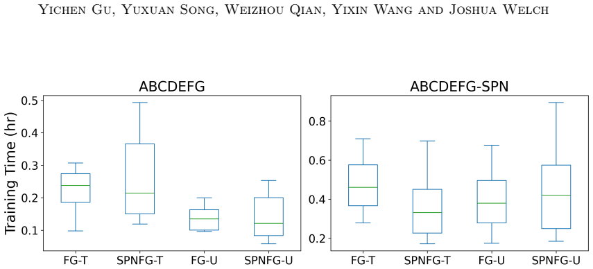
Kevin Bello, Bryon Aragam, and Pradeep Ravikumar. Dagma: Learning dags via m-matrices and a log-determinant acyclicity characterization. In S. Koyejo, S. Mohamed, 45 Yichen Gu, Yuxuan Song, Weizhou Qian, Yixin W ang and Joshua Welch Figure 15: Training Time of ABCDEFG.Each box represents one type of simulation. We group simulation regarding the ground tru...
2022
-
[5]
Variational dag estimation via state augmentation with stochastic permutations
Edwin V Bonilla, Pantelis Elinas, He Zhao, Maurizio Filippone, Vassili Kitsios, and Terry O’Kane. Variational dag estimation via state augmentation with stochastic permutations. arXiv preprint arXiv:2402.02644, 2024
arXiv 2024
-
[6]
Differentiable causal discovery from interventional data.Advances in Neural Information Processing Systems, 33:21865–21877, 2020
Philippe Brouillard, Sébastien Lachapelle, Alexandre Lacoste, Simon Lacoste-Julien, and Alexandre Drouin. Differentiable causal discovery from interventional data.Advances in Neural Information Processing Systems, 33:21865–21877, 2020
2020
-
[7]
Differentiable DAG sampling
Bertrand Charpentier, Simon Kibler, and Stephan Günnemann. Differentiable DAG sampling. InInternational Conference on Learning Representations, 2022
2022
-
[8]
iSCAN: Identifying causal mechanism shifts among nonlinear additive noise models
Tianyu Chen, Kevin Bello, Bryon Aragam, and Pradeep Kumar Ravikumar. iSCAN: Identifying causal mechanism shifts among nonlinear additive noise models. InThirty- seventh Conference on Neural Information Processing Systems, 2023. URL https: //openreview.net/forum?id=GEtXhqKW6X
2023
-
[9]
Bcd nets: Scalable variational approaches for bayesian causal discovery.Advances in Neural Information Processing Systems, 34:7095–7110, 2021
Chris Cundy, Aditya Grover, and Stefano Ermon. Bcd nets: Scalable variational approaches for bayesian causal discovery.Advances in Neural Information Processing Systems, 34:7095–7110, 2021
2021
-
[10]
Deep end-to-end causal inference
Tomas Geffner, Javier Antoran, Adam Foster, Wenbo Gong, Chao Ma, Emre Kiciman, Amit Sharma, Angus Lamb, Martin Kukla, Nick Pawlowski, Agrin Hilmkil, Joel Jennings, Meyer Scetbon, Miltiadis Allamanis, and Cheng Zhang. Deep end-to-end causal inference. Transactions on Machine Learning Research, 2024. ISSN 2835-8856
2024
-
[11]
Bacadi: Bayesian causal discovery with unknown 46 Amortized Bayesian Causal Discovery of Extended F actor Graphs interventions
Alexander Hägele, Jonas Rothfuss, Lars Lorch, Vignesh Ram Somnath, Bernhard Schölkopf, and Andreas Krause. Bacadi: Bayesian causal discovery with unknown 46 Amortized Bayesian Causal Discovery of Extended F actor Graphs interventions. InInternational Conference on Artificial Intelligence and Statistics, pages 1411–1436. PMLR, 2023
2023
-
[12]
Categorical reparameterization with gumbel- softmax
Eric Jang, Shixiang Gu, and Ben Poole. Categorical reparameterization with gumbel- softmax. InInternational Conference on Learning Representations, 2017
2017
-
[13]
Kingma andMax Welling
Diederik P. Kingma andMax Welling. Auto-encodingvariational bayes. In YoshuaBengio and Yann LeCun, editors,2nd International Conference on Learning Representations, ICLR 2014, Banff, AB, Canada, April 14-16, 2014, Conference Track Proceedings, 2014
2014
-
[14]
Scaling structural learning with no-bears to infer causal transcriptome networks
Hao-Chih Lee, Matteo Danieletto, Riccardo Miotto, Sarah T Cherng, and Joel T Dudley. Scaling structural learning with no-bears to infer causal transcriptome networks. In Pacific Symposium on Biocomputing 2020, pages 391–402. World Scientific, 2019
2020
-
[15]
Efficient neural causal discovery without acyclicity constraints
Phillip Lippe, Taco Cohen, and Efstratios Gavves. Efficient neural causal discovery without acyclicity constraints. InInternational Conference on Learning Representations, 2022
2022
-
[16]
Pritchard, and Aviv Regev
Romain Lopez, Jan-Christian Hütter, Jonathan K. Pritchard, and Aviv Regev. Large- scale differentiable causal discovery of factor graphs. InAdvances in Neural Information Processing Systems, 2022
2022
-
[17]
Stable differentiable causal discovery
Achille Nazaret, Justin Hong, Elham Azizi, and David Blei. Stable differentiable causal discovery. In Ruslan Salakhutdinov, Zico Kolter, Katherine Heller, Adrian Weller, Nuria Oliver, Jonathan Scarlett, and Felix Berkenkamp, editors,Proceedings of the 41st International Conference on Machine Learning, volume 235 ofProceedings of Machine Learning Research,...
2024
-
[18]
Jonas Peters and Peter Bühlmann. Structural intervention distance for evaluating causal graphs.Neural Computation, 27(3):771–799, 03 2015. ISSN 0899-7667. doi: 10.1162/NECO_a_00708. URLhttps://doi.org/10.1162/NECO_a_00708
-
[19]
Sum-product networks: A new deep architecture
Hoifung Poon and Pedro Domingos. Sum-product networks: A new deep architecture. In 2011 IEEE International Conference on Computer Vision Workshops (ICCV Workshops), pages 689–690. IEEE, 2011
2011
-
[20]
SoftSort: A continuous relaxation for the argsort operator
Sebastian Prillo and Julian Eisenschlos. SoftSort: A continuous relaxation for the argsort operator. In Hal Daumé III and Aarti Singh, editors,Proceedings of the 37th International Conference on Machine Learning, volume 119 ofProceedings of Machine Learning Research, pages 7793–7802. PMLR, 13–18 Jul 2020
2020
-
[21]
R. W. Robinson. Counting unlabeled acyclic digraphs. In Charles H. C. Little, editor, Combinatorial Mathematics V, pages 28–43, Berlin, Heidelberg, 1977. Springer Berlin Heidelberg. ISBN 978-3-540-37020-8
1977
-
[22]
Probabilistic circuits for variational inference in discrete graphical models.Advances in neural information processing systems, 33:4635–4646, 2020
Andy Shih and Stefano Ermon. Probabilistic circuits for variational inference in discrete graphical models.Advances in neural information processing systems, 33:4635–4646, 2020. 47 Yichen Gu, Yuxuan Song, Weizhou Qian, Yixin W ang and Joshua Welch
2020
-
[23]
An algorithm for fast recovery of sparse causal graphs
Peter Spirtes and Clark Glymour. An algorithm for fast recovery of sparse causal graphs. Social Science Computer Review, 9(1):62–72, 1991
1991
-
[24]
DeepITE: Designing variational graph autoencoders for intervention target estimation
Hongyuan Tao, Hang Yu, and Jianguo Li. DeepITE: Designing variational graph autoencoders for intervention target estimation. InThe Thirty-eighth Annual Conference on Neural Information Processing Systems, 2024. URL https://openreview.net/ forum?id=GMsi9966DR
2024
-
[25]
Ryan Thompson, Edwin V Bonilla, and Robert Kohn. Prodag: Projection-induced variational inference for directed acyclic graphs.arXiv preprint arXiv:2405.15167, 2024
arXiv 2024
-
[26]
Characterizing and learning equiva- lence classes of causal DAGs under interventions
Karren Yang, Abigail Katcoff, and Caroline Uhler. Characterizing and learning equiva- lence classes of causal DAGs under interventions. In Jennifer Dy and Andreas Krause, editors,Proceedings of the 35th International Conference on Machine Learning, vol- ume 80 ofProceedings of Machine Learning Research, pages 5541–5550. PMLR, 10–15 Jul 2018
2018
-
[27]
Learning unknown interven- tion targets in structural causal models from heterogeneous data
Yuqin Yang, Saber Salehkaleybar, and Negar Kiyavash. Learning unknown interven- tion targets in structural causal models from heterogeneous data. In Sanjoy Das- gupta, Stephan Mandt, and Yingzhen Li, editors,Proceedings of The 27th Inter- national Conference on Artificial Intelligence and Statistics, volume 238 ofProceed- ings of Machine Learning Research...
2024
-
[28]
Low-rank regularization for learning gene expression programs.PloS one, 8(12):e82146, 2013
Guibo Ye, Mengfan Tang, Jian-Feng Cai, Qing Nie, and Xiaohui Xie. Low-rank regularization for learning gene expression programs.PloS one, 8(12):e82146, 2013
2013
-
[29]
Dags with no curl: An efficient dag structure learning approach
Yue Yu, Tian Gao, Naiyu Yin, and Qiang Ji. Dags with no curl: An efficient dag structure learning approach. In Marina Meila and Tong Zhang, editors,Proceedings of the 38th International Conference on Machine Learning, volume 139 ofProceedings of Machine Learning Research, pages 12156–12166. PMLR, 18–24 Jul 2021
2021
-
[30]
Dags with no tears: Continuous optimization for structure learning
Xun Zheng, Bryon Aragam, Pradeep K Ravikumar, and Eric P Xing. Dags with no tears: Continuous optimization for structure learning. In S. Bengio, H. Wallach, H. Larochelle, K. Grauman, N. Cesa-Bianchi, and R. Garnett, editors,Advances in Neural Information Processing Systems, volume 31. Curran Associates, Inc., 2018
2018
-
[31]
Low-rank graph- regularized structured sparse regression for identifying genetic biomarkers.IEEE Trans- actions on Big Data, 3(4):405–414, 2017
Xiaofeng Zhu, Heung-Il Suk, Heng Huang, and Dinggang Shen. Low-rank graph- regularized structured sparse regression for identifying genetic biomarkers.IEEE Trans- actions on Big Data, 3(4):405–414, 2017. 48
2017
discussion (0)
Sign in with ORCID, Apple, or X to comment. Anyone can read and Pith papers without signing in.