REVIEW 2 major objections 3 minor 38 references
The paper's central claim: a 3D Gaussian splatting model trained on rendered images compresses a 281-million-particle snapshot by 65x while preserving visual fidelity and enabling real-time parameter changes.
Reviewed by Pith at T0; open to challenge. T0 means a machine referee read the full paper against a public rubric. the ladder, T0–T4 →
ParticleGS uses 3D Gaussian splats to mimic ParaView renderings of 281M-particle data, reaching 30 dB PSNR at 65x compression and rendering at 662 FPS.
T0 review reviewed 2026-08-01 challenge →
load-bearing objection A genuinely useful, honestly scoped visualization-aware compression pipeline for particle data; the main evaluation gap is that VizMapper's parameter adaptation is validated only by Beta-sampled averages, not a within-range parameter grid. the 2 major comments →
3D Gaussian Splatting for Scientific Particle Data Compression and Rendering
The pith
A machine-rendered reading of the paper's core claim, the machinery that carries it, and where it could break.
The reading
Core claim
The paper's central claim is that a compact set of anisotropic 3D Gaussians, about 769 thousand for a 281-million-particle snapshot, can be optimized end-to-end to stand in for the original particle set for interactive density visualization. The optimization target is not coordinate error but the pixel-wise difference between the Gaussian render and the reference renderer's pointsplat image, with a small adaptation network (VizMapper) that rescales each Gaussian's size and transparency when the user changes particle radius or opacity. The paper reports that this single trained model, after KD-tree spatial blocking and global fine-tuning, reaches 30.03 dB PSNR at 65x compression, generalizes
What carries the argument
The load-bearing object is the 3D Gaussian representation: each particle structure is encoded as a Gaussian with a center, covariance, opacity, and color, and rendering is a differentiable alpha-compositing of projected Gaussians. The paper adds VizMapper, a 4,610-parameter MLP that maps the user's radius/opacity change plus each Gaussian's own scale/opacity to multiplicative corrections, letting one model adapt to arbitrary settings at inference. A multi-orbit, progressive-resolution schedule with a content-masked L1 loss trains the model; KD-tree spatial blocking with per-block training, a coordinate-frame merge, and global fine-tuning scales capacity to 281M particles; and opacity-weighte
Load-bearing premise
The entire method stands or falls on whether the reference renderer's point-splat images across the trained radius/opacity/camera range can be faithfully reproduced by alpha-composited 3D Gaussians with only global multiplicative scale/opacity corrections.
What would settle it
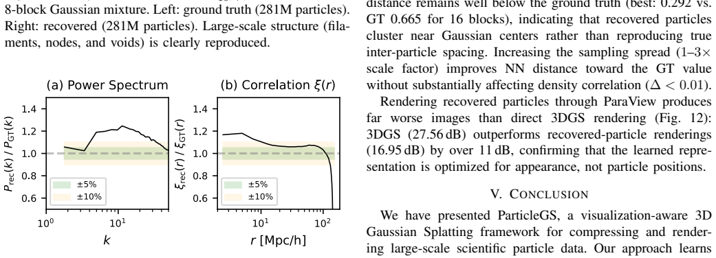
Render the reference point-splatting output at a held-out (r, α) pair inside the training envelope, e.g., r≈0.014, α≈0.02, from a camera at 0.7x orbit, and compare to the VizMapper-adapted 3DGS render; if masked PSNR drops materially below the trained-orbit level or errors concentrate along filament boundaries, the multiplicative-correction assumption is wrong. Alternatively, sample recovered particles and check the power spectrum: failure to stay within ±10% of the ground truth P(k) up to k≈2.63 h/Mpc would falsify the density-surrogate claim.
If this is right
- A 49.8 MB Gaussian model can replace a 3.4 GB particle snapshot for interactive density-field visualization, at 65x compression and 30 dB PSNR.
- User changes to particle radius and opacity cost about 1.2 ms per frame instead of a full re-render over hundreds of millions of particles, putting parameter exploration into interactive territory.
- The same trained pipeline, without dataset-specific tuning, reaches 27–29 dB PSNR at 264–577x compression on other cosmological regions and on a snapshot from a different simulation code.
- Particle positions recovered from the Gaussian mixture preserve large-scale clustering statistics, including a power spectrum within about 10% to k≈2.63 h/Mpc, but not nearest-neighbor or other small-scale structure, so the representation is suitable for density-domain analysis only.
- Training costs 67 minutes on a single GPU; after that, rendering runs at over 600 FPS at 1080p while using under half a gigabyte of GPU memory.
Where Pith is reading between the lines
- If the density-surrogate interpretation is right, this approach turns scientific data compression into a renderer-matching problem: any renderer with a differentiable image model could be targeted, with the same pipeline retrained on that renderer's output.
- The reported compression ratio should not be compared with general error-bounded compressors for tasks requiring exact coordinates; the paper's own scope caveat makes the representation a visualization format, not a general-purpose particle data format.
- The sub-linear growth of Gaussian count with particle count suggests the block-training scheme may scale toward far larger snapshots, but only if per-block fine-tuning remains feasible and boundary artifacts stay controlled, both untested beyond 281M particles.
- A cheap testable extension: benchmark VizMapper-adapted renderings against the reference renderer on a dense grid of radius/opacity pairs beyond the Beta-sampled training range; the reported smooth degradation outside the envelope suggests graceful, but still unquantified, limits.
Editorial analysis
A structured set of objections, weighed in public.
Referee Report
Summary. The paper proposes ParticleGS, a 3D Gaussian Splatting framework for compressing large-scale particle data into a compact set of Gaussians optimized for rendered image quality rather than point-wise data fidelity. The method combines a multi-orbit, multi-resolution training schedule; VizMapper, a small MLP that adapts Gaussian scale and opacity to user-specified particle radius and opacity at inference time; and KD-tree spatial block training with global fine-tuning. On a 281M-particle HACC snapshot, the 8-block model reports 30.03 dB PSNR at 65x compression, outperforming SZ3 by 5–8 dB and LCP by larger margins, generalizing to other HACC regions and FIRE-2 without per-dataset tuning, and rendering at 662 FPS. The paper also describes approximate particle recovery via GMM sampling, with explicit statements that only large-scale density statistics are preserved.
Significance. If the claims hold, this is a practically valuable, visualization-oriented compressed representation for particle data, with real-time rendering and explicit support for interactive parameter changes. The paper has notable strengths: consistent ablations that isolate the contribution of each component; a block-training analysis with sensible scaling behavior; generalization tests across datasets from two different simulation codes; and an unusually honest discussion of scope, especially in Section IV-H and the Conclusion, which clearly delineate what the representation can and cannot support. The GMM-recovery experiments, with P(k) and two-point correlation checks, go beyond visual metrics and help establish appropriate use. The artifact link and the detailed experimental configuration are positive elements. However, the central 'single model adapts to user parameters' claim needs stronger validation than the current mean-PSNR-over-Beta-samples evidence, and the headline quantitative results would be more convincing with repeated-run statistics.
major comments (2)
- [Section III-B, Eqs. (3)–(4); Section IV-E, Table V] The central claim that one trained model adapts to arbitrary user radius/opacity changes without retraining rests on VizMapper's multiplicative scale/opacity form. The only in-range validation is mean PSNR over per-frame (r, alpha) drawn from Beta(3,3), a distribution concentrated near the defaults; Section IV-E's extrapolation tests use only a few points (f_r=2.0, 2.5; f_alpha=2.0, 2.4). Because training samples parameters from the same Beta distribution, an average over that distribution can hide large errors at edge combinations (e.g., r near 0.0025 with alpha near 0.0875). Please add a dense within-range grid (e.g., 5x5 or 6x6 over r in [0.0025, 0.0175] and alpha in [0.0125, 0.0875]) comparing VizMapper-adapted 3DGS renders against ParaView ground truth, reporting per-cell PSNR and worst-case error, and include the static-model baseline for comparison. This experiment is directly loa
- [Section IV-A, Tables IV and VI] Headline numbers (28.80 dB single-block, 30.03 dB 8-block, 27.36±0.04 dB generalization) are reported as single runs. Training involves random Beta-sampled radius/opacity, random camera orbits, and stochastic 3DGS densification; without a fixed seed or repeated runs, the reported dB differences could be within run-to-run variation. Please report mean±std over at least three seeds for the primary HACC operating points and for the FIRE-2 result, or state and provide the fixed seeds used in the artifact. This matters because the paper's quantitative claims (e.g., +5.4 dB over SZ3) depend on the precision of these numbers.
minor comments (3)
- [Section III-C vs. Table II] The text says 'Adding DSSIM ... inflates model size by 68% without improving masked PSNR,' but Table II shows pure DSSIM at 298.2 MB versus 49.8 MB (about 6x) and L1+0.1 DSSIM at 54.2 MB (about 9% larger). Please reconcile or specify which configuration the 68% figure refers to.
- [Table II] The 'w/o densification' row reports a larger size (57.9 MB) than the production recipe (49.8 MB), while the text says the merged model 'needs new Gaussians to fill gaps between block boundaries.' If the larger size is due to the absence of pruning, please say so explicitly; otherwise the row is confusing.
- [Figure 2 vs. Abstract] Figure 2 states '665 FPS' while the abstract and Table VII state 662 FPS. Please align the numbers.
Circularity Check
No significant circularity: the derivation is a supervised image-fitting pipeline with independent held-out, extrapolation, and external-baseline validation.
full rationale
The paper's central result is a learned representation optimized directly to reproduce ParaView point-Gaussian renderings, and it is evaluated with exactly that objective (masked L1 during training, PSNR during evaluation). This proximity is the stated design goal rather than a concealed reuse: the training loss and evaluation metric are different instantiations of the same image fidelity target, and the paper does not present the training objective as an independent prediction. Crucially, the evaluation includes held-out generalization evidence that breaks any fitted-input/prediction equivalence: unseen camera orbits (Section IV-E, Table V), out-of-range radius/opacity factors with smooth degradation, spatially disjoint HACC snapshots, and a different simulation code (FIRE-2) all use the default pipeline without tuning. The comparisons against SZ3 and LCP are external baselines rendered through the same ParaView pipeline, and the particle-recovery analysis (Section IV-H) is validated against the original particle data using density correlation, power spectrum, and nearest-neighbor distances, giving independent grounding outside the rendering objective. VizMapper's multiplicative correction form is an architectural assumption, not a circular step, and the paper explicitly discloses its scope and limitations (Section V), including the visual-fidelity ceiling, the trained-envelope restriction, and the density-only nature of particle recovery. Self-citations to prior work by the same authors (SZ3, LCP, HPEZ-family compressors) appear only as baselines or related work, not as load-bearing justification for the paper's claims. No equation in the paper reduces by construction to a fitted value, and no uniqueness theorem or ansatz is imported from the authors' prior work. The manuscript is self-contained against external benchmarks and honestly delineates where the representation is and is not trustworthy.
Axiom & Free-Parameter Ledger
free parameters (6)
- Training radius/opacity sampling ranges and Beta concentration =
r in [0.0025,0.0175], alpha in [0.0125,0.0875], beta=3.0
- Multi-orbit/resolution training schedule =
3 orbits (1.0/0.7/0.5x), 12k+27k iterations, 1920x1080 then 5760x3240, 20% interior cameras
- VizMapper input normalization constants (mu_s, Delta_s, mu_o, Delta_o) =
estimated from a pilot run on a reference dataset; exact values not reported
- VizMapper correction bounds (delta_max_s, delta_max_o, epsilon) =
0.1/0.3/0.4 initially; 0.3/0.8/0.1 after merge
- Block count K =
8 for the primary result; 2, 4, 16 also tested
- Inherited 3DGS hyperparameters =
not reported; 'same densification configuration' as standard 3DGS
axioms (7)
- domain assumption ParaView's Point Gaussian rendering is an adequate ground-truth oracle for scientific visualization quality, and L1 loss against these images preserves structures scientists care about.
- ad hoc to paper User-adjusted radius/opacity changes are fully captured by multiplicative correction of Gaussian scale and opacity (Eqs. 3-4).
- domain assumption A diffuse mixture of ~171k-769k 3D Gaussians can represent the density field of 281M particles well enough for visual PSNR > 28 dB, and 3DGS adaptive densification finds such a mixture.
- domain assumption KD-tree block decomposition, affine merging, and global fine-tuning repair inter-block seams without requiring retraining from scratch.
- domain assumption Opacity of learned Gaussians is proportional to local particle density, allowing GMM weight sampling for approximate particle recovery.
- domain assumption Beta sampling of radius and opacity during training represents the distribution of real user exploration; results outside this envelope are not guaranteed.
- standard math The standard differentiable 3DGS rasterizer correctly composites semi-transparent Gaussians front-to-back.
Cite this review
Pith. "Pith review of 3D Gaussian Splatting for Scientific Particle Data Compression and Rendering." pith.science (2026). https://pith.science/paper/CTVW2GIF
@misc{pith2026260722956,
  author       = {Pith},
  title        = {Pith review of: 3D Gaussian Splatting for Scientific Particle Data Compression and Rendering},
  year         = {2026},
  howpublished = {\url{https://pith.science/paper/CTVW2GIF}},
  note         = {Machine review of arXiv:2607.22956}
}
read the original abstract
Large-scale particle simulations produce hundreds of millions of particles, straining storage, transfer, and interactive visualization. Existing lossy compressors such as SZ3 operate in data space and provide no guarantees on downstream visualization fidelity. We propose ParticleGS, a visualization-aware framework based on 3D Gaussian Splatting (3DGS) that learns a compact representation directly optimized for rendered image quality, combining (1) a multi-stage, multi-orbit training pipeline, (2) VizMapper, a lightweight network that adapts a single trained model to user-specified visualization parameters at inference time, and (3) spatial block training with KD-tree decomposition and global fine-tuning. On a 281-million-particle HACC cosmological simulation, our 8-block model reaches 30.03 dB PSNR at 65x compression, outperforming SZ3 by 5-8 dB at comparable ratios, and generalizes without tuning to additional HACC regions and a dark-matter-only FIRE-2 simulation. It renders at 662 FPS on a single GPU, over 2,300x faster than ParaView on the full particle data.
Figures



Reference graph
Works this paper leans on
-
[1]
HACC: Simulating sky surveys on state-of-the-art supercomputing architectures,
S. Habib, A. Pope, H. Finkel, N. Frontiere, K. Heitmann, D. Daniel, P. Fasel, V . Morozov, G. Zagaris, T. Peterkaet al., “HACC: Simulating sky surveys on state-of-the-art supercomputing architectures,”New Astronomy, vol. 42, pp. 49–65, 2016. [Online]. Available: https: //doi.org/10.1016/j.newast.2015.06.003
-
[2]
FIRE-2 simulations: physics versus numerics in galaxy formation,
P. F. Hopkins, A. Wetzel, D. Kere ˇs, C.-A. Faucher-Gigu`ere, E. Quataert, M. Boylan-Kolchin, N. Murray, C. C. Hayward, S. Garrison-Kimmel, C. Hummelset al., “FIRE-2 simulations: physics versus numerics in galaxy formation,”Monthly Notices of the Royal Astronomical Society, vol. 480, no. 1, pp. 800–863, 2018. [Online]. Available: https://doi.org/10.1093/m...
-
[3]
Public data release of the FIRE-2 cosmological zoom-in simulations of galaxy formation,
A. Wetzel, C. C. Hayward, R. E. Sanderson, X. Ma, D. Angl ´es- Alc´azar, R. Feldmann, T. Chan, K. El-Badry, C. Wheeler, S. Garrison- Kimmelet al., “Public data release of the FIRE-2 cosmological zoom-in simulations of galaxy formation,”The Astrophysical Journal Supplement Series, vol. 265, no. 2, p. 44, 2023
2023
-
[4]
A. P. Thompson, H. M. Aktulga, R. Berger, D. S. Bolintineanu, W. M. Brown, P. S. Crozier, P. J. In’t Veld, A. Kohlmeyer, S. G. Moore, T. D. Nguyenet al., “LAMMPS—a flexible simulation tool for particle-based materials modeling at the atomic, meso, and continuum scales,”Computer physics communications, vol. 271, p. 108171, 2022. [Online]. Available: https:...
arXiv 2022
-
[5]
Paraview: An end-user tool for large data visualization,
J. Ahrens, B. Geveci, and C. Law, “Paraview: An end-user tool for large data visualization,”The visualization handbook, vol. 717, no. 8,
-
[6]
Fast error-bounded lossy hpc data compression with sz,
S. Di and F. Cappello, “Fast error-bounded lossy hpc data compression with sz,” in2016 ieee international parallel and distributed processing symposium (ipdps). IEEE, 2016, pp. 730–739. [Online]. Available: https://doi.org/10.1109/IPDPS.2016.11
-
[7]
SZ3: A modular framework for composing prediction-based error-bounded lossy compressors,
X. Liang, K. Zhao, S. Di, S. Li, R. Underwood, A. M. Gok, J. Tian, J. Deng, J. C. Calhoun, D. Taoet al., “SZ3: A modular framework for composing prediction-based error-bounded lossy compressors,”IEEE Transactions on Big Data, vol. 9, no. 2, pp. 485–498, 2022. [Online]. Available: https://doi.org/10.1109/TBDATA.2022.3201176
arXiv 2022
-
[8]
Fixed-rate compressed floating-point arrays,
P. Lindstrom, “Fixed-rate compressed floating-point arrays,”IEEE transactions on visualization and computer graphics, vol. 20, no. 12, pp. 2674–2683, 2014. [Online]. Available: https://doi.org/10.1109/ TVCG.2014.2346458
arXiv 2014
-
[9]
Q. Gong, J. Chen, B. Whitney, X. Liang, V . Reshniak, T. Banerjee, J. Lee, A. Rangarajan, L. Wan, N. Vidalet al., “MGARD: A multigrid framework for high-performance, error-controlled data compression and refactoring,”SoftwareX, vol. 24, p. 101590, 2023. [Online]. Available: https://doi.org/10.1016/j.softx.2023.101590
arXiv 2023
-
[10]
Lcp: Enhancing scientific data management with lossy compression for particles,
L. Zhang, R. Li, C. Ren, S. Di, J. Liu, J. Huang, R. Underwood, P. Grosset, D. Tao, X. Lianget al., “Lcp: Enhancing scientific data management with lossy compression for particles,”Proceedings of the ACM on Management of Data, vol. 3, no. 1, pp. 1–27, 2025. [Online]. Available: https://doi.org/10.1145/3709700
doi:10.1145/3709700 2025
-
[11]
Compressive neural representations of volumetric scalar fields,
Y . Lu, K. Jiang, J. A. Levine, and M. Berger, “Compressive neural representations of volumetric scalar fields,” inComputer graphics forum, vol. 40, no. 3. Wiley Online Library, 2021, pp. 135–146. [Online]. Available: https://doi.org/10.1111/cgf.14295
-
[12]
J. Han and C. Wang, “CoordNet: Data generation and visualization generation for time-varying volumes via a coordinate-based neural network,”IEEE Transactions on Visualization and Computer Graphics, vol. 29, no. 12, pp. 4951–4963, 2022. [Online]. Available: https: //doi.org/10.1109/TVCG.2022.3197203
arXiv 2022
-
[13]
NeRF: Representing scenes as neural radiance fields for view synthesis,
B. Mildenhall, P. P. Srinivasan, M. Tancik, J. T. Barron, R. Ramamoorthi, and R. Ng, “NeRF: Representing scenes as neural radiance fields for view synthesis,”Communications of the ACM, vol. 65, no. 1, pp. 99–106, 2021. [Online]. Available: https://doi.org/10.1145/3503250
doi:10.1145/3503250 2021
-
[14]
Fast neural representations for direct volume rendering,
S. Weiss, P. Herm ¨uller, and R. Westermann, “Fast neural representations for direct volume rendering,” inComputer Graphics Forum, vol. 41, no. 6. Wiley Online Library, 2022, pp. 196–211. [Online]. Available: https://doi.org/10.1111/cgf.14578
-
[15]
S. Yao, Y . Lu, and C. Wang, “ViSNeRF: Efficient multidimensional neural radiance field representation for visualization synthesis of dynamic volumetric scenes,” in2025 IEEE 18th Pacific Visualization Conference (PacificVis). IEEE, 2025, pp. 235–245. [Online]. Available: https://doi.org/10.1109/PacificVis64226.2025.00029
arXiv 2025
-
[16]
An algebraic process for visualization design,
G. Kindlmann and C. Scheidegger, “An algebraic process for visualization design,”IEEE transactions on visualization and computer graphics, vol. 20, no. 12, pp. 2181–2190, 2014. [Online]. Available: https://doi.org/10.1109/TVCG.2014.2346325
arXiv 2014
-
[17]
3D Gaussian Splatting for real-time radiance field rendering,
B. Kerbl, G. Kopanas, T. Leimk ¨uhler, and G. Drettakis, “3D Gaussian Splatting for real-time radiance field rendering,”ACM Transactions on Graphics, vol. 42, no. 4, July 2023. [Online]. Available: https://doi.org/10.1145/3592433
doi:10.1145/3592433 2023
-
[18]
Simulating cosmic structure formation with the Gadget-4 code,
V . Springel, R. Pakmor, O. Zier, and M. Reinecke, “Simulating cosmic structure formation with the Gadget-4 code,”Monthly Notices of the Royal Astronomical Society, vol. 506, no. 2, pp. 2871–2949, 2021. [Online]. Available: https://doi.org/10.1093/mnras/stab1855
-
[19]
TTHRESH: Tensor compression for multidimensional visual data,
R. Ballester-Ripoll, P. Lindstrom, and R. Pajarola, “TTHRESH: Tensor compression for multidimensional visual data,”IEEE transactions on visualization and computer graphics, vol. 26, no. 9, pp. 2891–2903,
-
[20]
J. Liu, S. Di, K. Zhao, X. Liang, S. Jin, Z. Jian, J. Huang, S. Wu, Z. Chen, and F. Cappello, “High-performance effective scientific error-bounded lossy compression with auto-tuned multi- component interpolation,”Proceedings of the ACM on Management of Data, vol. 2, no. 1, pp. 1–27, 2024. [Online]. Available: https://doi.org/10.1145/3639259
-
[21]
cuSZ: An efficient gpu-based error-bounded lossy compression framework for scientific data,
J. Tian, S. Di, K. Zhao, C. Rivera, M. H. Fulp, R. Underwood, S. Jin, X. Liang, J. Calhoun, D. Taoet al., “cuSZ: An efficient gpu-based error-bounded lossy compression framework for scientific data,” inProceedings of the ACM International Conference on Parallel Architectures and Compilation Techniques, 2020, pp. 3–15. [Online]. Available: https://doi.org/...
arXiv 2020
-
[22]
CUSZ-i: High-ratio scientific lossy compression on gpus with optimized multi-level interpolation,
J. Liu, J. Tian, S. Wu, S. Di, B. Zhang, R. Underwood, Y . Huang, J. Huang, K. Zhao, G. Liet al., “CUSZ-i: High-ratio scientific lossy compression on gpus with optimized multi-level interpolation,” inSC24: International Conference for High Performance Computing, Networking, Storage and Analysis. IEEE, 2024, pp. 1–15. [Online]. Available: https://doi.org/1...
Pith/arXiv arXiv 2024
-
[23]
In-depth exploration of single-snapshot lossy compression techniques for n-body simulations,
D. Tao, S. Di, Z. Chen, and F. Cappello, “In-depth exploration of single-snapshot lossy compression techniques for n-body simulations,” in2017 IEEE International Conference on Big Data (Big Data). IEEE, 2017, pp. 486–493. [Online]. Available: https://doi.org/10.1109/ BigData.2017.8257962
arXiv 2017
-
[24]
Dynamic quality metric oriented error bounded lossy compression for scientific datasets,
J. Liu, S. Di, K. Zhao, X. Liang, Z. Chen, and F. Cappello, “Dynamic quality metric oriented error bounded lossy compression for scientific datasets,” inSC22: International Conference for High Performance Computing, Networking, Storage and Analysis. IEEE, 2022, pp. 1–15. [Online]. Available: https://doi.org/10.1109/SC41404.2022.00067
Pith/arXiv arXiv 2022
-
[25]
Toward quantity-of-interest preserving lossy compression for scientific data,
P. Jiao, S. Di, H. Guo, K. Zhao, J. Tian, D. Tao, X. Liang, and F. Cappello, “Toward quantity-of-interest preserving lossy compression for scientific data,” Argonne National Laboratory (ANL), Tech. Rep.,
-
[26]
Exploring autoencoder-based error-bounded compression for scientific data,
J. Liu, S. Di, K. Zhao, S. Jin, D. Tao, X. Liang, Z. Chen, and F. Cappello, “Exploring autoencoder-based error-bounded compression for scientific data,” in2021 IEEE International Conference on Cluster Computing (CLUSTER). IEEE, 2021, pp. 294–306. [Online]. Available: https://doi.org/10.1109/Cluster48925.2021.00034
arXiv 2021
-
[27]
Z-checker: A framework for assessing lossy compression of scientific data,
D. Tao, S. Di, H. Guo, Z. Chen, and F. Cappello, “Z-checker: A framework for assessing lossy compression of scientific data,”The International Journal of High Performance Computing Applications, vol. 33, no. 2, pp. 285–303, 2019. [Online]. Available: https: //doi.org/10.1177/1094342017737147
-
[28]
Instant neural graphics primitives with a multiresolution hash encoding,
T. M ¨uller, A. Evans, C. Schied, and A. Keller, “Instant neural graphics primitives with a multiresolution hash encoding,”ACM transactions on graphics (TOG), vol. 41, no. 4, pp. 1–15, 2022. [Online]. Available: https://doi.org/10.1145/3528223.3530127
arXiv 2022
-
[29]
Mip-splatting: Alias-free 3D Gaussian splatting,
Z. Yu, A. Chen, B. Huang, T. Sattler, and A. Geiger, “Mip-splatting: Alias-free 3D Gaussian splatting,” inProceedings of the IEEE/CVF conference on computer vision and pattern recognition, 2024, pp. 19 447–19 456. [Online]. Available: https://doi.org/10.48550/arXiv.2311. 16493
-
[30]
Compact 3D Gaussian representation for radiance field,
J. C. Lee, D. Rho, X. Sun, J. H. Ko, and E. Park, “Compact 3D Gaussian representation for radiance field,” inProceedings of the IEEE/CVF Conference on Computer Vision and Pattern Recognition, 2024, pp. 21 719–21 728. [Online]. Available: https: //doi.org/10.48550/arXiv.2311.13681
-
[31]
Mini-splatting: Representing scenes with a constrained number of Gaussians,
G. Fang and B. Wang, “Mini-splatting: Representing scenes with a constrained number of Gaussians,” inEuropean conference on computer vision. Springer, 2024, pp. 165–181. [Online]. Available: https://doi.org/10.48550/arXiv.2403.14166
-
[32]
4D Gaussian splatting for real-time dynamic scene rendering,
G. Wu, T. Yi, J. Fang, L. Xie, X. Zhang, W. Wei, W. Liu, Q. Tian, and X. Wang, “4D Gaussian splatting for real-time dynamic scene rendering,” inProceedings of the IEEE/CVF conference on computer vision and pattern recognition, 2024, pp. 20 310–20 320. [Online]. Available: https://doi.org/10.48550/arXiv.2310.08528
-
[33]
VastGaussian: Vast 3D Gaussians for Large Scene Reconstruction
J. Lin, Z. Li, X. Tang, J. Liu, S. Liu, J. Liu, Y . Lu, X. Wu, S. Xu, Y . Yanet al., “VastGaussian: Vast 3D gaussians for large scene reconstruction,” inProceedings of the IEEE/CVF Conference on Computer Vision and Pattern Recognition, 2024, pp. 5166–5175. [Online]. Available: https://doi.org/10.48550/arXiv.2402.17427
work page internal anchor Pith review Pith/arXiv arXiv doi:10.48550/arxiv.2402.17427 2024
-
[34]
Image quality assessment: from error visibility to structural similarity,
Z. Wang, A. C. Bovik, H. R. Sheikh, and E. P. Simoncelli, “Image quality assessment: from error visibility to structural similarity,”IEEE transactions on image processing, vol. 13, no. 4, pp. 600–612, 2004. [Online]. Available: https://doi.org/10.1109/TIP.2003.819861
arXiv 2004
-
[35]
P. J. E. Peebles,The large-scale structure of the universe. Princeton University Press, 2020. [Online]. Available: https://doi.org/10.23943/ princeton/9780691209838.001.0001
arXiv 2020
-
[2005]
Available: https://doi.org/10.1016/B978-012387582-2% 2F50038-1
[Online]. Available: https://doi.org/10.1016/B978-012387582-2% 2F50038-1
-
[2019]
Available: https://doi.org/10.1109/TVCG.2019.2904063
[Online]. Available: https://doi.org/10.1109/TVCG.2019.2904063
arXiv 2019
-
[2022]
Available: https://doi.org/10.14778/3574245.3574255
[Online]. Available: https://doi.org/10.14778/3574245.3574255
This paper was first reviewed by deepseek-v4-flash on August 1, 2026.
discussion (0)
Sign in with ORCID, Apple, or X to comment. Anyone can read and Pith papers without signing in.