REVIEW 4 major objections 10 minor 23 references
Minimal FNO changes—hypernetwork shift modulation plus Fourier-space coupling—cut errors 55–72% on parameterized coupled PDEs while keeping standard FNO size and cost.
Reviewed by Pith at T0; open to challenge. T0 means a machine referee read the full paper against a public rubric. the ladder, T0–T4 →
T0 review · grok-4.5
2026-07-30 21:30 UTC pith:XXP3SBAQ
load-bearing objection Solid incremental FNO engineering paper: lightweight parameter shifts plus a clear coupled-design checklist, real gains on a new plasma benchmark, but the 55–72% headline sits on thin test splits and selective low-Tin seeds. the 4 major comments →
Extending Fourier Neural Operators for Modeling Parameterized and Coupled PDEs
The pith
A machine-rendered reading of the paper's core claim, the machinery that carries it, and where it could break.
Core claim
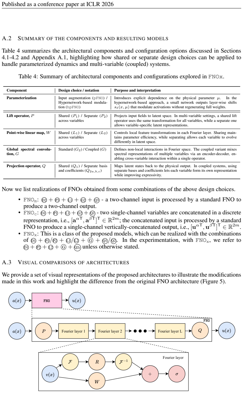
Principled minimal extensions of FNOs—hypernetwork-generated shift modulation for physical parameters together with a specific coupled layout (shared lift, separate pointwise linear maps, Fourier-domain encoder–decoder coupling, and fully separate projection bases and coefficients)—yield up to 55–72% lower normalized RMSE than strong baselines on parameterized coupled time-dependent PDEs, without materially increasing model size or per-epoch cost.
What carries the argument
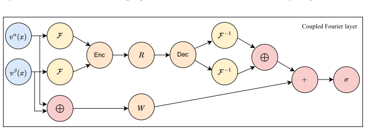
hpFNOx: a compact hypernetwork that outputs layer-wise additive shifts s_ℓ(x,μ) inserted as biases inside the Fourier layers, combined with spectral-domain coupling that mixes the Fourier coefficients of the variables through shallow encoder/decoder maps while leaving the rest of the FNO structure intact.
Load-bearing premise
The claimed gains rest on short history windows plus fixed initial conditions, and on reporting only the best half of runs when those windows shrink to one or two steps.
What would settle it
Retrain every model on the same CCP and Gray–Scott splits with Tin = 1 using all random seeds (no best-of-10 filtering) and check whether hpFNOx still shows a clear, stable error reduction versus the strongest non-parameterized baseline.
If this is right
- Surrogate models for plasma etch/deposition tools can condition on voltage, reaction rate and ion mass without retraining a new operator for each setting.
- The same shared-lift / separate-projection / Fourier-space-mix pattern can be dropped into other spectral neural operators with little extra code.
- When only a single initial snapshot is available, explicit parameter modulation becomes necessary; history windows alone are insufficient.
- The simplified 1-D CCP system supplies a public, multi-parameter coupled benchmark for future operator-learning work.
Where Pith is reading between the lines
- The same shift-modulation idea should transfer to other operator families (DeepONet, multiwavelet, attention-based) whenever the task is parameterized dynamics from a fixed initial state.
- If the Fourier-space encoder–decoder is replaced by a cheap cross-attention block, the architecture may scale more gracefully past two or four fields.
- Reporting full multi-seed statistics at Tin = 1 would turn the low-history regime into a sharper stress test for any parameter-conditioned operator.
Editorial analysis
A structured set of objections, weighed in public.
Referee Report
Summary. The manuscript proposes two minimal extensions of Fourier neural operators: (i) hpFNO, in which a lightweight hypernetwork conditioned on the physical parameter vector µ produces layer-wise shift (bias) modulations of the Fourier-layer activations, and (ii) FNOx, a coupled-system architecture obtained from a systematic design-space exploration over the lift, pointwise map, spectral convolution, and projection operators, with cross-variable coupling confined to Fourier space via a shallow linear encoder–decoder. The recommended configuration is P1+L2+G⃝+Q2c with layer normalization. The methods are evaluated on a new 1D capacitively coupled plasma (CCP) benchmark (varying reaction rate R0, driving voltage V0, ion mass mi, plus a 2D parameter grid), the Gray–Scott system (varying diffusion and feed rate), and a 2D four-field reacting-flow case in the appendix. Against baselines (FNOc/m, CFNO, MWTc, CMWNO, HyperFNOc-T/A, DONc, U-Netc), the proposed variants reduce nRMSE by up to ~55% (CCP) and ~72% (Gray–Scott feed rate) relative to the strongest baseline, at model size and per-epoch cost comparable to standard FNOs. A Tin sweep argues the parametric variants degrade gracefully as the input history window shrinks.
Significance. If the results hold, this is a useful and practical contribution. The fixed-initial-condition, parameterized-PDE regime is genuinely underserviced in the operator-learning literature, and the paper's strengths are real: a controlled comparison in which all FNO-family baselines share identical depth/modes/width (4 layers, k=12, dv=20, App. B.1) so gains are attributable to architecture rather than capacity; a systematic ablation over the coupling design space (Table 6); five-seed mean±std reporting throughout; explicit model-size and per-epoch timing accounting (Figs. 4, 12, 16); an OOD parameter-strip study (Table 8, Fig. 14); resolution-robustness checks (Fig. 17); and a physically motivated new CCP benchmark with documented governing equations, solver, and parameter ranges (App. C), which is a genuine community asset. The shift-modulation mechanism is simple, cheap, and shown to be competitive with or better than full-weight HyperFNO variants, and the negative result on naive multiplicative gating with a stabilized tanh fix (Table 10) is honestly reported. The central comparative claim — that the hpFNOx family outperforms strong baselines at Tin=10 — is supported by margins (e.g.
major comments (4)
- [§5.2.2, Table 2] Table 2, footnote ‡: for Tin∈{2,1} the paper trains 10 seeds and reports the mean over the best 5 by test accuracy. This is selection on the test metric and biases both the mean and the std downward; the reported 13–16% relative errors for the hp variants are therefore optimistic by an unknown amount. This matters because the low-Tin / initial-condition-only regime is the paper's stated practical motivation ('only initial conditions are available in most practical setups', §5.2.2). The fix is cheap: report all 10 seeds (or the median and full range), and separately report the failure/divergence rate, which is itself informative about the deployment story. As written, the load-bearing low-Tin numbers do not support the deployment claim.
- [§5.2.1, Tables 1, 3, 9, 11] The headline margins rest on very small test sets, and the reported error bars capture only training-seed variance, not test-set sampling. Each 1D CCP experiment uses 100 equidistant parameter configurations with a 9:1 split (§5.2.1), i.e. ~10 test trajectories; Gray–Scott uses 101 samples (App. E.1); the 2D reacting-flow case has 8 test trajectories (App. F.1). Since the parameter grids are equidistant and the split is random, a single split can over- or under-represent stiff regions (e.g. the high-R0 end, Fig. 10). Nothing in Tables 1, 2, 3, 9, or 11 quantifies sensitivity to which parameters landed in the test set. Given that some margins are small relative to plausible test-set sampling noise (e.g. hpFNOx 0.0124 vs pFNOx 0.0140 in Table 9), the authors should repeat the train/test split over multiple draws (or use a stratified split) and report variance across splits, at least for th
- [§1 / §5.3 / App. E.1] The paper is framed throughout as addressing parameterized dynamics with fixed initial conditions (§1: 'u_t = f(u;µ) with u(0)=u0'; §5.2.1: 'A fixed initial condition is used'), but the Gray–Scott experiments sample a fresh random initial condition per trajectory — u(x,0) from Chebfun smooth random functions and v(x,0) from a Gaussian random field (App. E.1). These are different regimes: with varying ICs, the operator must additionally disambiguate IC from parameter effects, and the fixed-IC motivation (and the Tin delay-embedding argument of §5.2.2) does not directly apply. The authors should clarify which trajectories share ICs, and reconcile the framing; if the Gray–Scott ICs vary, the claim that the method targets the fixed-IC regime should be scoped to the CCP experiments.
- [§4.3, App. A.2, App. B.1, Table 6] There is an internal inconsistency in the definition of the FNOx design point, and the single largest ablation gain comes from a component absent from the design space. §4.3 defines FNOx as P1+L2+G⃝+Q2c; App. A.2 states FNOx is 'D1+P2+L2+G⃝+Q2c unless otherwise stated'; App. B.1 reverts to P1+L2+Q2c 'obtained from the ablation study'. Meanwhile Table 6 shows the chosen configuration is P1+L2+Q2c with layer norm, and the layer norm contributes the largest single improvement in the table (0.0275→0.0193), exceeding the gain from any coupling design choice (P1+L1+Q1 → P1+L2+Q2c gives 0.0341→0.0275). Layer normalization appears nowhere in the design-space taxonomy of §4.2/App. A, so the claim that 'performance gains can be attributed to structural insights rather than increased capacity' (§4) is only partially supported — a nontrivial fraction of the gain is a training/normalization tweak app
minor comments (10)
- [App. D.1.3, Table 10] Table 10 is captioned as applied to hpFNOc, but the 'Shift only' row (0.0154/0.0279/0.0128) matches the hpFNOc column of Table 7 only for two of three columns, and 0.0154/0.0128 match hpFNOx in Table 1; please verify which model the table reports and make the caption consistent.
- [§4.1 vs App. B.1] App. B.1 states the hypernetwork takes (x, µ) 'along with the discrete representation of the windowed history {u(t−τ)}', which contradicts §4.1 where s(x,µ)=fhyper(x,µ) depends only on the parameter and position. If the shifts are also functions of the solution history, hpFNO is closer to a second lift operator than to pure parameter conditioning; please clarify the actual inputs.
- [§5.2 / App. C.1, Eq. (14)] Eq. (14): the drift flux is written Γe = −D∂x ne + µ ne ∂xφ with µ>0; with E=−∂xφ the electron drift flux would conventionally be −µ ne ∂xφ. Please confirm the sign convention used in the solver (or note if the model is defined as written), since readers from plasma physics will check this.
- [App. B.1] App. B.1, CMWNO dice description: 'the first operator takes the first operator's hidden representation' — one of these should be 'second operator'.
- [App. C.1, Table 5] Table 5: 'Reaction rage coefficients' → 'rate'; there is also a stray apostrophe in the R0 range '[2.7×10^19, 2.7×10^20‘]'.
- [Abstract / §5.3] The '55–72%' figures in the abstract aggregate different baselines per case (e.g. 55% is vs CFNO on driving voltage; 72–76% is vs MWTc on Gray–Scott feed rate). Stating the reference baseline for each number would make the claims easier to verify.
- [App. D.1.3] The OOD study (Table 8, Fig. 14) is a nice addition, but with only 10 OOD samples per side the per-parameter curves in Fig. 14 carry substantial uncertainty; a sentence on sample size would calibrate the reader.
- [§8 / App. C] Reproducibility: code release is promised only 'upon acceptance' (§8). Given that all baseline configurations and solver details are otherwise well documented, an anonymized repository at submission time would strengthen the paper; at minimum, please specify the finite-difference scheme used to generate the CCP data (App. C currently says only 'finite-difference solver').
- [§4.2 / App. A] Notation: the coupled spectral operator is rendered as G⃝ throughout, which does not survive PDF extraction and is easy to confuse with the standard G2; consider a plain symbol (e.g. Gc).
- [App. D.1.3, Fig. 15] Figure 15 reports improvement over a dbasis=8 baseline but the absolute nRMSE values are not given; adding an absolute-error axis would make the orthogonality-loss effect (~10% at small basis) easier to interpret alongside λortho selection (App. B.3).
Circularity Check
No significant circularity: empirical supervised operator learning on held-out PDE trajectories; architectural choices and hypernetwork shifts are fitted parameters, not identities forced by definition.
full rationale
The paper’s load-bearing claims are comparative nRMSE reductions of proposed FNO variants (hpFNOx, pFNOx, FNOx) versus baselines on held-out parameter configurations of 1D CCP, Gray–Scott, and a 2D reacting-flow system. Training is standard supervised operator learning: discrete-time evolution maps are fit to numerical trajectories and evaluated with normalized RMSE on test splits (9:1 random splits of equidistant parameter grids). Hypernetwork shift modulation and the coupled design space (shared lift, separate W, Fourier-space encoder–decoder, separate Q bases/coefficients) are architectural hypotheses whose weights are optimized against data; the reported “predictions” are next-state PDE fields, not algebraic rearrangements of the fitted inputs. Architecture selection via ablation (Appendix D.1.1 / Table 6) on one CCP setting before reuse elsewhere is ordinary model selection, not a self-definitional reduction. Related-work citations (HyperFNO, CMWNO, FiLM, etc.) supply baselines and motivation; none is a uniqueness theorem by overlapping authors that forces the claimed architecture. There is no closed-form derivation equating outputs to inputs by construction, no fitted scalar renamed as a first-principles prediction, and no self-citation chain that substitutes for external evidence. Circularity score is therefore 0.
Axiom & Free-Parameter Ledger
free parameters (5)
- FNO depth/modes/width (4 layers, k=12, dv=20) =
4 layers, 12 modes, width 20
- Hypernetwork architecture (linear baseline; depth/width variants) =
linear layer primary; MLP variants reported
- Tin history window and selective seed reporting at Tin∈{1,2} =
Tin default 10; best-5-of-10 at Tin=1,2
- Orthogonality loss weight λ_ortho and scale-modulation amplitude η =
λ_ortho in {0.1,0.01,0.001}; η in {0.1,0.5}
- Optimizer and schedule hyperparameters =
lr 0.0025 (DON 1e-4), wd 1e-4, batch 10
axioms (5)
- domain assumption Neural operators trained as one-step maps with autoregressive rollout approximate the discrete-time PDE flow from a finite history window.
- domain assumption 1D CCP model with constant ion density, prescribed reaction zones, and sinusoidal boundary voltage is a representative surrogate target for sheath dynamics.
- ad hoc to paper Cross-variable coupling restricted to Fourier space via shallow linear encoder–decoder is sufficient to capture interactions while preserving FNO efficiency.
- domain assumption Fixed initial condition across parameter instances is the practical regime of interest versus jointly varying ICs and parameters.
- standard math Standard supervised L2/nRMSE on normalized fields is the right success metric for operator quality.
invented entities (3)
-
hpFNO / hpFNOx (hypernetwork shift-modulated coupled FNO)
no independent evidence
-
FNOx design point (P1+L2+G⃝+Q2c)
no independent evidence
-
1D capacitively coupled plasma (CCP) operator-learning benchmark
no independent evidence
read the original abstract
Parameterized and coupled partial differential equations (PDEs) are central to modeling phenomena in science and engineering, yet neural operator methods that address both aspects remain limited. We extend Fourier neural operators (FNOs) with minimal architectural modifications along two directions. For parameterized dynamics, we propose a hypernetwork-based modulation that conditions the operator on physical parameters. For coupled systems, we conduct a systematic exploration of architectural choices, examining how operator components can be adapted to balance shared structure with cross-variable interactions while retaining the efficiency of standard FNOs. Evaluations on benchmark PDEs, including the one-dimensional capacitively coupled plasma equations and the Gray-Scott system, show that our methods achieve up to 55-72% lower errors than strong baselines, demonstrating the effectiveness of principled modulation and systematic design exploration.
Figures








Reference graph
Works this paper leans on
-
[1]
HyperFNO: Improving the general- ization behavior of Fourier neural operators
Francesco Alesiani, Makoto Takamoto, and Mathias Niepert. HyperFNO: Improving the general- ization behavior of Fourier neural operators. InNeurIPS 2022 Workshop on Machine Learning and Physical Sciences,
2022
-
[2]
Sharing main- tains parameter efficiency, while separating allows each variable to evolve differently in latent space
across variables Controls local feature transformations in each Fourier layer. Sharing main- tains parameter efficiency, while separating allows each variable to evolve differently in latent space. Global spectral convolu- tion,G Standard (G2) / Coupled (G) Defines non-local interactions in Fourier space. The coupled variant mixes spectral representations...
2026
-
[3]
Benjamin Holzschuh, Qiang Liu, Georg Kohl, and Nils Thuerey. PDE-Transformer: Efficient and versatile transformers for physics simulations.arXiv preprint arXiv:2505.24717,
-
[7]
Zongyi Li, Nikola Kovachki, Kamyar Azizzadenesheli, Burigede Liu, Kaushik Bhattacharya, An- drew Stuart, and Anima Anandkumar. Neural operator: Graph kernel network for partial differ- ential equations.arXiv preprint arXiv:2003.03485, 2020a. Zongyi Li, Nikola Kovachki, Kamyar Azizzadenesheli, Burigede Liu, Andrew Stuart, Kaushik Bhat- tacharya, and Anima ...
Pith/arXiv arXiv 2003
-
[8]
While the proposedhpFNO x exhibits a mild degradation at the largestν m, it still achieves the lowest overall errors (nRMSE≈0.015–0.018)
As summarized in Figure 13a, we observe a general trend of increasing nRMSE with higherν m across all models. While the proposedhpFNO x exhibits a mild degradation at the largestν m, it still achieves the lowest overall errors (nRMSE≈0.015–0.018). This behavior is consistent with the underlying plasma physics: as the system becomes more col- lisional, ele...
2026
-
[9]
Detecting strange attractors in turbulence
Floris Takens. Detecting strange attractors in turbulence. InDynamical Systems and Turbulence, Warwick 1980: proceedings of a symposium held at the University of Warwick 1979/80, pp. 366–
1980
-
[10]
Each variable is treated as an independent function,a(x) = (aα(x), aβ(x)), and discretized separately asa α,a β ∈R m
13 Published as a conference paper at ICLR 2026 A DESIGN SPACES OFFNOS A.1 DESCRIPTION ON EACH COMPONENT Data space D1 Separate single-channel format. Each variable is treated as an independent function,a(x) = (aα(x), aβ(x)), and discretized separately asa α,a β ∈R m. This representation keeps the two components distinct throughout the architecture. D2 Tw...
2026
-
[11]
Q2 The projection operator is defined separately for each output component,Q= (Q α, Qβ), with Q□ :R dv →R 1 for□∈ {α, β}. From the adaptive-basis perspective,Qcan differ in whether the basis and the coefficients are shared or separate across the two variables: • Q2a Shared basis and separate coefficients, and • Q2b Separate basis and shared coefficients, ...
2026
-
[12]
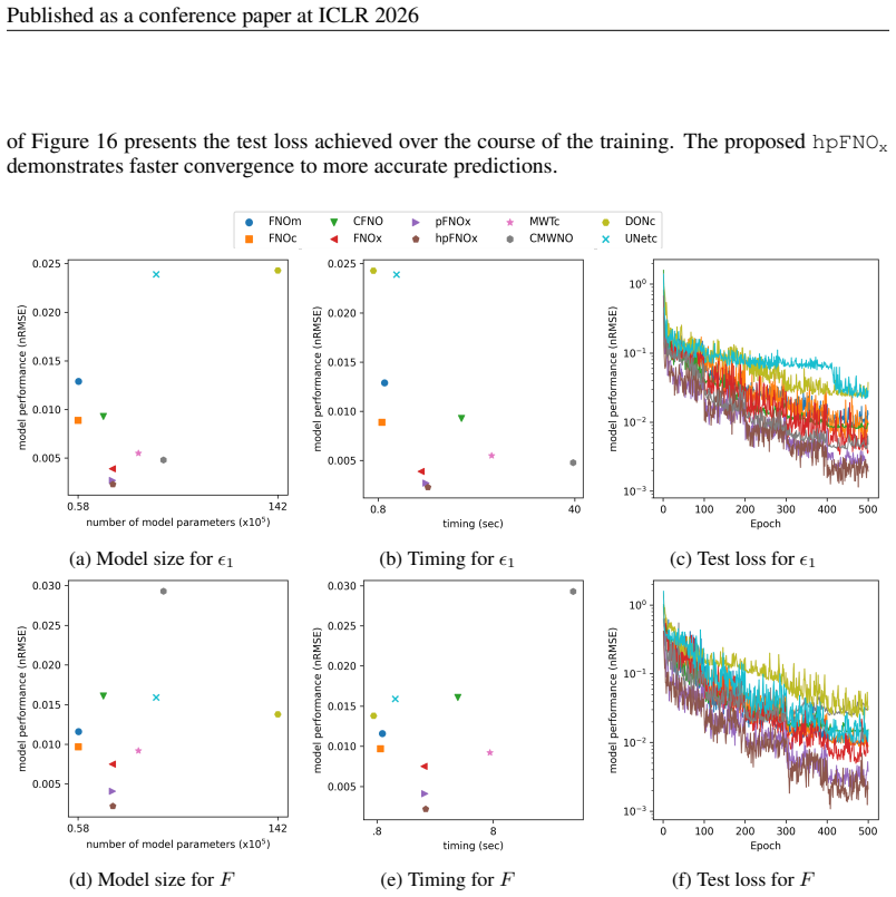
This time, the information obtained from the experimentation with the datasets that vary the reaction rate and the ion masses. Again, the model size is measured in the number of trainable model parameters and the timing reports a per-epoch training time measured and averaged across the total number of epochs. We can make the similar observations here: the...
2026
-
[14]
The scaling parameterαis set to 12, the channel multipliercis set to 16, the wavelet polynomial order cis set to 4, and the base polynomial basis is set to the ‘Legendre’ polynomials. The dice strategy 2https://github.com/joshuaxiao98/CMWNO/ 18 Published as a conference paper at ICLR 2026 is utilized as follows: for each batch we throw a random number fro...
2026
-
[15]
,(11) whereT in decides the window length. The trunk net is modeled as a separate network, producing two separate sets of basis such that [f trunk,ne (x), ftrunk,ϕ(x)] = [W ne f trunk(x) +b ne , Wϕf trunk(x) +b nϕ ],(12) wheref trunk denotes a shared MLP, and(W ne, bne )and(W ϕ, bnϕ )denote a set of model parameters specific to the electron density and el...
2026
-
[16]
For U-Nets, we consider the same hyperparameters, except for the total training epochs, which is set to 1,000, which is to mitigate the effect of the increased model sizes. For DeepONets, we again consider the same hyperparameters, except for the learning rate, which is set to 0.0001 and the total training epochs, which is set to 2,500 which is to compens...
2026
-
[17]
All Figures present the two spatio-temporal fields, the electron densityn e(x, t)and the electric potentialϕ(x, t), in thet−xplane, in a heatmap format
in the first RF cycle. All Figures present the two spatio-temporal fields, the electron densityn e(x, t)and the electric potentialϕ(x, t), in thet−xplane, in a heatmap format. Figure 10 shows the solution snapshots for varying reaction ratesR 0 ={2.7×10 19,1.485× 1020,2.7×10 20}m−3s−1. The reaction rate serves as a quantity that determines how fast ion- i...
2026
-
[20]
Table 8 reports the performance of all considered models on ID test samples and OOD test samples
For training, 101 equidistant values of the reaction rate is sampled from [2.7×10 19, 2.7×10²⁰]; for OOD testing, the interval is expanded outward by 0.2×10 19 in both directions. Table 8 reports the performance of all considered models on ID test samples and OOD test samples. Overall, the performance measured on OOD produces increased numbers, but the tr...
2024
-
[23]
Table 11: Performance comparisons between the proposed methods and the baseline methods
The time integration is performed for the time interval [0,0.1] with 31 time steps. Table 11: Performance comparisons between the proposed methods and the baseline methods. All models are tested on a scalar parameter: the diffusion coefficient. The performance is measured in the relativeℓ 2-error; the reported numerical values refer to the mean (±standard...
2026
-
[128]
In the experiments described in the main body, we consider the Taylor variant; in the Appendix, we provide the results of both variants
In the Taylor form, the modulation is expressed through a first-order expansion around the base parameters: hR(θℓ R, µ) =Rℓ 0 ⊙ I+V ℓ R diag(hR,µ(µ))V ℓ R ⊤ , h W (θℓ W , µ) =W ℓ 0 ⊙ I+U ℓ W hW,µ(µ) , (9) where⊙denotes element-wise multiplication. In the experiments described in the main body, we consider the Taylor variant; in the Appendix, we provide th...
2023
-
[256]
Deeper or narrower configurations, such as a 3-layer network (width 256, nRMSE = 0.0200) or 3- layer network (width 32, nRMSE = 0.0230), show a mild degradation in performance
and 1 hidden layer (width 128), which yield nRMSE values in the range of 0.0171-0.0179 compared to 0.0154 for the linear baseline. Deeper or narrower configurations, such as a 3-layer network (width 256, nRMSE = 0.0200) or 3- layer network (width 32, nRMSE = 0.0230), show a mild degradation in performance. These results indicate thathpFNO x performance is...
2018
-
[2014]
and samplingv(x,0)from Gaussian random field, v(x,0)∼ N(0,7 4(−2π+ 7 2I) −2.75). For collecting trajectories for constructing training/test datasets, initial value problems are numerically solved using a fourth-order time-integrator, expo- nential time differencing fourth-order Runge–Kutta (ETDRK4), utilizing the chebfun software. We base the implementati...
2023
-
[2015]
URLhttps: //arxiv.org/abs/1412.6980. 11 Published as a conference paper at ICLR 2026 Nikola Kovachki, Zongyi Li, Burigede Liu, Kamyar Azizzadenesheli, Kaushik Bhattacharya, An- drew Stuart, and Anima Anandkumar. Neural operator: Learning maps between function spaces with applications to PDEs.Journal of Machine Learning Research, 24(89):1–97,
Pith/arXiv arXiv 2026
-
[2021]
Kingma and Jimmy Ba
Diederik P. Kingma and Jimmy Ba. Adam: A method for stochastic optimization. InProceedings of the 3rd International Conference on Learning Representations (ICLR 2015),
2015
-
[2023]
URLhttps: //openreview.net/forum?id=j3oQF9coJd
ISSN 2835-8856. URLhttps: //openreview.net/forum?id=j3oQF9coJd. 12 Published as a conference paper at ICLR 2026 Md Ashiqur Rahman, Robert Joseph George, Mogab Elleithy, Daniel Leibovici, Zongyi Li, Boris Bonev, Colin White, Julius Berner, Raymond A Yeh, Jean Kossaifi, et al. Pretraining codomain attention neural operators for solving multiphysics PDEs.Adv...
2026
-
[2024]
Projection-based model reduction for reacting flows
10 Published as a conference paper at ICLR 2026 Marcelo Buffoni and Karen Willcox. Projection-based model reduction for reacting flows. In40th Fluid Dynamics Conference and Exhibit, pp. 5008,
2026
-
[2025]
The Sol supercomputer at Arizona State University
Douglas M Jennewein, Johnathan Lee, Chris Kurtz, William Dizon, Ian Shaeffer, Alan Chapman, Alejandro Chiquete, Josh Burks, Amber Carlson, Natalie Mason, et al. The Sol supercomputer at Arizona State University. InPractice and Experience in Advanced Research Computing 2023: Computing for the Common Good, pp. 296–301
2023
discussion (0)
Sign in with ORCID, Apple, or X to comment. Anyone can read and Pith papers without signing in.