REVIEW 3 major objections 8 minor 69 references
A single statewide deep learning model can detect emerging crash hotspots, forecast next week’s risk maps, and track each hotspot’s life cycle before enforcement trails the cycle.
Reviewed by Pith at T0; open to challenge. T0 means a machine referee read the full paper against a public rubric. the ladder, T0–T4 →
T0 review · grok-4.5
2026-07-31 22:02 UTC pith:CNONWMEE
load-bearing objection Solid applied systems paper with a real emergence head; the headline win over baselines is mostly the exposure anchor the others never got, so scope the claim before you lean on the leaderboard. the 3 major comments →
Forecasting the Emergence and Evolution of Crash Hotspots: A Unified Deep Learning Framework for Proactive Traffic Safety
The pith
A machine-rendered reading of the paper's core claim, the machinery that carries it, and where it could break.
Core claim
HERALD establishes that emerging-hotspot detection, short-term intensity and centroid forecasting, and interpretable life-cycle tracking can be driven from one shared spatial–temporal representation and one statewide model, attaining the best macro grid-level error among five matched baselines while leading hotspot F1 and centroid displacement across six heterogeneous counties and flagging emergent risk before it consolidates.
What carries the argument
HERALD: a compact CNN–Transformer with a regime-routed mixture-of-experts that forecasts weekly multi-channel crash grids by composing an exposure-anchored background risk with Hawkes-style self-excitation under a zero-inflated negative-binomial head, then matches clusters over time into birth–growth–stable–decline–death trajectories.
Load-bearing premise
The model treats a static map built only from each county’s past crash intensities as a trustworthy stand-in for true long-run exposure and risk geography.
What would settle it
Retrain and evaluate on counties or years with a sharp shift in traffic, network layout, or enforcement (for example after major construction or a new patrol regime); if grid accuracy and hotspot F1 fall behind baselines that do not lean on the historical crash-exposure anchor, the claim of portable proactive forecasting fails.
If this is right
- Agencies can run one statewide model instead of separate tools for clustering, forecasting, and tracking.
- Ranking quiet cells by the birth head can capture a large share of next-week injuries that static exposure maps miss.
- One amplitude calibration knob lets operators choose accuracy-first or sensitivity-first deployment per county.
- Five-phase life-cycle labels give a readable timeline for when to intervene and when to stand down.
- Dense urban and sparse rural regimes can share weights via mixture-of-experts without per-county retraining.
Where Pith is reading between the lines
- If the exposure anchor mostly replays where crashes already concentrate, reported gains may shrink when true traffic volume, weather, or network inventory is added as a competing prior.
- The same three-task substrate—detection, short-horizon forecast, and life-cycle matching—could transfer to crime or disease clusters where sparse counts and near-repeat excitation also dominate.
- Closing the loop from life-cycle phases into digital-twin or connected-vehicle timing, as the authors sketch, would turn forecasts into scheduled interventions rather than maps alone.
Editorial analysis
A structured set of objections, weighed in public.
Referee Report
Summary. The paper introduces HERALD, a statewide deep-learning pipeline that jointly (i) forecasts next-week severity-stratified crash-injury grids on a 50×50 tessellation, (ii) emits explicit hotspot centroids plus an emergence ("birth") probability head for historically quiet cells, and (iii) tracks DBSCAN clusters through a five-phase life cycle via Hungarian matching. The architecture is a compact (0.38M-parameter) CNN encoder + factorized axial transformer with a density-routed two-expert mixture, a FiLM county modulation, and a structured intensity head that multiplicatively anchors on a training-window exposure map (Eq. 22) with a Hawkes-style excitation term and a hurdle/NB likelihood. On six Wisconsin counties (2018–2020) with chronological per-county splits, HERALD reports the best macro MAE (0.0215 vs. 0.0241 for the next-best CNN), best macro F1@2km (0.409) and displacement (0.644 km) among five baselines trained under a shared protocol, and a birth head that captures 11.3% of emergent injuries in the top 1% of flagged quiet cells on Dane.
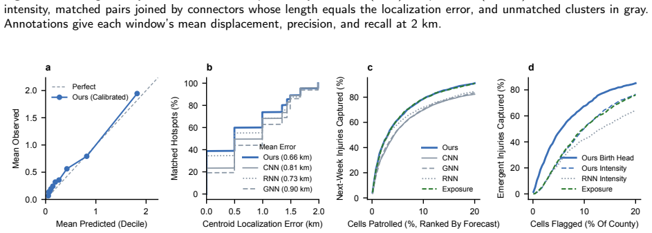
Significance. If the results hold, this is a useful contribution to proactive traffic-safety analytics: a single small model serving heterogeneous density regimes, an explicit and well-motivated separation of grid-error metrics from localization metrics, an operationally meaningful early-warning product (emergent-injury capture, Fig. 9d), and an interpretable life-cycle tracker. The evaluation practices deserve explicit credit: chronological per-county splits, an identical training recipe across baselines, per-county breakdowns over two orders of magnitude in density, a genuine leave-one-out component analysis (Table 4), a disclosed post-hoc calibration with fitted scales reported, and an unusually candid correction that the likelihood is hurdle-style rather than mixture ZINB (§3.2.9). The exposure anchor's nature as a crash-history proxy rather than true exposure is also stated openly (§3.1.4). However, the central comparative claim currently rests on an input asymmetry the manuscript does not close (see Major 1), and uncertainty quantification is absent.
major comments (3)
- [§3.1.4, §3.2.4, Eq. (22), Tables 2–4, Fig. 9(c)] The headline claim 'outperforms five identically trained baselines' is not currently separable from 'is the only model given the long-run mean.' Per §4.1.2, all six models share the dynamic channels (severity, cluster field, cyclicity; history k=4 weeks), while the static exposure/occupancy maps (§3.2.4) and the unit-coupling E_c anchor (Eq. 22) are HERALD-only inputs. E_c is the per-cell mean over ~110 training windows — information the baselines cannot reconstruct from 4 weeks of history. The paper's own Table 4 makes the attribution explicit: removing the anchor moves macro MAE to 0.0245 (behind the CNN's 0.0241) and macro F1 to 0.231 (behind RNN 0.379, LSTM 0.397); Fig. 9(c) concedes the static exposure ranking ties HERALD on overall injury capture. Two controls are needed before the comparative claim can stand: (a) a non-learned climatology row in Tables 2–3 (forecast = calibrated E
- [§3.2.10, §4.1.2] All results are reported under a single fixed random seed, with no confidence intervals or significance tests, even though Fig. 6 already computes per-window metric distributions. Several headline margins are small and could plausibly be seed- or window-noise: macro MAE 0.0215 vs. 0.0241, and per-county MAE gaps in sparse counties are tiny in absolute terms (Sauk 0.0043 vs. 0.0052; Chippewa 0.0026 vs. 0.0034). Given that training takes ~3 minutes on a consumer GPU, multi-seed runs (e.g., 5–10 seeds) are inexpensive; alternatively, paired window-level tests (block bootstrap over test windows or a Diebold–Mariano test against the CNN) would directly address whether the MAE/F1 leads are statistically supported. This is load-bearing because the claim is a ranking, not an effect size.
- [§2.1, §4.1.1] The test period (final 31 windows per county, roughly June–December 2020) coincides with the COVID-19 disruption, which shifted traffic volumes, trip patterns, and crash severity mix statewide; the exposure anchor E_c is built from training windows dominated by pre-pandemic conditions. Since Major 1 establishes that the anchor carries the model's margin, its behavior under this known regime shift is directly load-bearing, yet the manuscript never mentions the pandemic. The within-period model comparison remains fair (all models face the same test weeks), so this does not invalidate the ranking; but the paper should (a) acknowledge the shift explicitly, (b) report whether weekly totals/CV in the test windows deviate from training (Table 1 covers the full period only), and (c) ideally split test results into early- vs. late-2020. If performance holds, this is a genuine robustness result wo
minor comments (8)
- [§4.4, Fig. 9(d)] Please add a chance-level reference line for emergent-injury capture (uniform ranking of quiet cells would capture ~1% at the 1% budget) and report emergent capture for at least one sparse county in addition to Dane, since early warning in sparse regimes is where the birth head would matter most operationally and where §4.5 reports its weakest performance.
- [§4.5] Life-cycle 'phase-classification accuracy' is measured against labels produced by running the same tracker (§3.3) on observed heatmaps, i.e., it quantifies forecast/observation consistency of a deterministic labeler, not correctness against independently validated life cycles. This is a reasonable proxy, but it should be stated explicitly in §4.5 and the abstract language ('produces temporally coherent life-cycle summaries') adjusted accordingly.
- [§3.2.10] The checkpoint-selection constants MAE0=0.0281 and RMSE0=0.2241 are described only as 'fixed reference constants'; state their provenance (e.g., a baseline's validation values) so the selection criterion is reproducible.
- [§3, notation] Grid-dimension notation is inconsistent: §3 opening defines a 'W×H tessellation' while most equations and §2.2 use H×W; also Eq. (4) uses W^s_t for intensity while W is the grid width, inviting confusion. A symbol table would help.
- [Table 1] Milwaukee's 183,907 injuries from 74,779 crashes (~2.46 injuries/crash, including PDO crashes) is surprisingly high; please verify whether 'injuries' counts persons injured across all severity tiers or something else, and define the quantity in the table caption.
- [Fig. 8] Cluster-geometry panels are drawn from 'the best-localized windows' (disclosed, which is good), but one or two median- or worst-case windows would give a more honest picture of typical geometry; at minimum, state the selection percentile.
- [Reproducibility] No code or data-availability statement is given. Given the many tuned components (loss weights, EMA decay, calibration grid, DBSCAN/matching thresholds), releasing training code and the county-grid preprocessing pipeline would substantially strengthen the paper; crash data restrictions should at least be acknowledged.
- [§3.2.7, Eq. (22)] The claim that fixing the anchor exponent at 1 comes 'at no cost to accuracy' is asserted without evidence; a one-line ablation with a learned exponent (or a citation) would support it, since this is the modeling choice at the center of Major 1.
Circularity Check
No significant circularity: held-out chronological evaluation and disclosed priors; main leaderboard claims are empirical, not definitional.
specific steps
-
fitted input called prediction
[§3.2.10 Training, Metric-Aligned Selection, and Output Calibration]
"a post-hoc output calibration corrects a systematic amplitude over-prediction of the zero-inflation–intensity product: one scalar per county, selected by grid search on that county’s validation windows to minimize MAE+RMSE, multiplies the expected intensity at inference. ... alongside the standard composite-loss checkpoint, a second checkpoint minimizes the validation error score MAE/MAE0 + RMSE/RMSE0"
A scalar (and optionally the checkpoint) is chosen on validation expressly to minimize the same MAE/RMSE family reported at test. This is ordinary metric-aligned calibration, not algebraic identity of prediction with input, and uses no test labels; it only mildly couples fitted amplitude to scored grid error. It does not make hotspot geometry or emergence rankings true by construction.
full rationale
HERALD is an empirical deep-learning systems paper, not a first-principles derivation. Grid forecasts, hotspot F1, and birth-head gains are scored on chronologically held-out future weeks against identically protocol-trained architectural baselines; nothing equates a reported prediction to its defining input by algebra. The static exposure map E_c (Eq. 7) is built from training-window crash means and enters the intensity head as a unit-coupling multiplicative anchor (Eq. 22)—a classical SPF-style prior the paper itself labels a crash-history proxy that “blends exposure with underlying risk.” That makes localization heavily prior-dependent (Table 4: −Exposure collapses macro F1 ~44%), and the missing climatology / exposure-augmented baseline is an attribution and fairness concern, not circularity of a derivation chain. Post-hoc per-county amplitude calibration and metric-aligned checkpointing on validation MAE/RMSE are standard and mild; they do not force test labels. Self-citations (digital twins, work zones, etc.) are peripheral, not load-bearing uniqueness theorems. Score 1 only for the mild val-fitted calibration touching reported error metrics; central claims remain independently falsifiable on held-out data.
Axiom & Free-Parameter Ledger
free parameters (7)
- Per-county output calibration scales =
0.4–0.6 per county
- NB dispersion r =
≈3.6
- Loss weights λ_MSE, λ_occ, λ_NB, λ_cent, λ_birth, λ_ord =
3 / 1 / 1 / 1 / 0.5 / 0.5
- History length k, grid size H×W, axial depth/width =
k=4, 50×50, d=96, L_a=2
- DBSCAN/match thresholds (ε=1 km, min_samples=1, gate=2 km, half-injury threshold) =
ε=1km; gate=2km; threshold=0.5 injury
- EMA decay and metric-aligned checkpoint rule =
EMA 0.998; MAE0=0.0281; RMSE0=0.2241
- Hawkes kernel and lag weights (9×9 K, w_κ, α severity mix) =
learned (~100 params)
axioms (7)
- domain assumption Weekly 50×50 county grids with k=4 history windows are an adequate discrete substrate for operational hotspot forecasting and tracking.
- ad hoc to paper Long-run crash-intensity maps are acceptable multiplicative exposure anchors (safety-performance-function style) even without VMT/road inventory.
- domain assumption Crash counts are over-dispersed and well modeled by a hurdle/zero-inflated negative-binomial factorization plus occupancy gate.
- domain assumption Recent crashes elevate nearby near-future risk via a discretized Hawkes-style triggering kernel.
- ad hoc to paper DBSCAN clusters on thresholded injury maps plus centroid matching within 2 km define operational ‘hotspots’ and localization truth.
- ad hoc to paper Dense-urban vs sparse-rural density regimes are the primary heterogeneity worth specializing via a two-expert router on exposure/occupancy/county embedding.
- domain assumption Chronological holdout within 2018–2020 Wisconsin six-county corpus is representative enough to support statewide deployment claims.
invented entities (4)
-
HERALD unified framework
no independent evidence
-
Regime-routed dense/sparse mixture-of-experts refinement
no independent evidence
-
Structured intensity head (exposure background + Hawkes excitation + hurdle NB)
no independent evidence
-
Five-phase hotspot life-cycle tracker (birth/growth/stable/decline/death)
no independent evidence
read the original abstract
Road crashes remain among the gravest threats to public safety, and preventing them is a defining task of transportation systems worldwide. Much of that harm concentrates at hotspots, yet a hotspot is less a place than an episode; it emerges quietly at an intersection or along an arterial, intensifies for weeks, then subsides, only to reappear elsewhere. Enforcement guided by maps of past crashes inevitably trails this cycle, patrolling yesterday's hotspots while tomorrow's form unwatched. Breaking that lag requires three capabilities at once: detecting hotspots as they are born, forecasting where they will sit next week, and following each one through its life. We introduce HERALD (Hotspot Emergence, Risk Anticipation, and Life-cycle Dynamics), a unified deep learning framework that provides all three from a single statewide model. HERALD distills each county's recent crash history into weekly risk maps and forecasts the next with a CNN--Transformer, whose mixture-of-experts lets one model serve dense urban cores and sparse rural corridors alike. Each forecast is anchored in the county's long-run crash geography, sharpened by the self-exciting effect of recent crashes, and paired with explicit warnings of where new hotspots are about to appear. Followed over time, every hotspot acquires a legible life story, from birth through growth and stability to decline and death. Across six heterogeneous Wisconsin counties, HERALD forecasts more accurately than five identically trained baselines, locates hotspots most precisely, and flags emerging risks before they take hold. A single adjustable setting trades accuracy for extra sensitivity where deployment demands it. The result shifts hotspot management from mapping the past to anticipating the future.
Figures




Reference graph
Works this paper leans on
-
[1]
W. H. Organization, Global status report on road safety 2023, World Health Organization, 2023
2023
-
[2]
M. M. Peden, World report on road traffic injury prevention, World Health Organization, 2004
2004
-
[3]
L.J.Blincoe,T.R.Miller,E.Zaloshnja,B.Lawrence,Theeconomicandsocietalimpactofmotorvehiclecrashes,2010(Revised),Technical Report DOT HS 812 013, National Highway Traffic Safety Administration, Washington, DC, 2015
2010
-
[4]
N.Corsaro,D.W.Gerard,R.S.Engel,J.E.Eck, Notbyaccident:Ananalyticalapproachtotrafficcrashharmreduction, JournalofCriminal Justice 40 (2012) 502–514. J. Zhu et al.:Preprint submitted to ElsevierPage 24 of 26 Forecasting the Emergence and Evolution of Crash Hotspots
2012
-
[5]
Elvik, A
R. Elvik, A. Høye, T. Vaa, M. Sørensen, The handbook of road safety measures, Emerald Group Publishing Limited, 2009
2009
-
[6]
Tingvall, N
C. Tingvall, N. Haworth, et al., Vision zero-an ethical approach to safety and mobility, in: 6th ITE international conference road safety & traffic enforcement: Beyond 2000, 1999
2000
-
[7]
M.-Å.Belin,P.Tillgren,E.Vedung, Visionzero–aroadsafetypolicyinnovation, Internationaljournalofinjurycontrolandsafetypromotion 19 (2012) 171–179
2012
-
[8]
E. Kim, P. Muennig, Z. Rosen, Vision zero: a toolkit for road safety in the modern era, Injury epidemiology 4 (2017) 1
2017
-
[9]
M.Abdel-Aty,N.Uddin,A.Pande,F.M.Abdalla,L.Hsia, Predictingfreewaycrashesfromloopdetectordatabymatchedcase-controllogistic regression, Transportation Research Record: Journal of the Transportation Research Board 1897 (2004) 88–95
2004
-
[10]
Getis, J
A. Getis, J. K. Ord, The analysis of spatial association by use of distance statistics, Geographical analysis 24 (1992) 189–206
1992
-
[11]
Z.Li,X.Cao,X.Gao,K.Tian,K.Wu,M.Anis,H.Zhang,K.Long,J.Jiang,X.Li,etal., Simulatingtheunseen:Crashpredictionmustlearn from what did not happen, arXiv preprint arXiv:2505.21743 (2025)
Pith/arXiv arXiv 2025
-
[12]
D. Lord, F. Mannering, The statistical analysis of crash-frequency data: A review and assessment of methodological alternatives, Transportation research part A: policy and practice 44 (2010) 291–305
2010
-
[13]
F. L. Mannering, C. R. Bhat, Analytic methods in accident research: Methodological frontier and future directions, Analytic methods in accident research 1 (2014) 1–22
2014
-
[14]
F. L. Mannering, V. Shankar, C. R. Bhat, Unobserved heterogeneity and the statistical analysis of highway accident data, Analytic methods in accident research 11 (2016) 1–16
2016
-
[15]
A. B. Parsa, A. Movahedi, H. Taghipour, S. Derrible, A. K. Mohammadian, Toward safer highways, application of xgboost and shap for real-time accident detection and feature analysis, Accident Analysis & Prevention 136 (2020) 105405
2020
-
[16]
Z. Xie, J. Yan, Kernel density estimation of traffic accidents in a network space, Computers, environment and urban systems 32 (2008) 396–406
2008
-
[17]
T.K.Anderson, Kerneldensityestimationandk-meansclusteringtoprofileroadaccidenthotspots, AccidentAnalysis&Prevention41(2009) 359–364
2009
-
[18]
W.Cheng,S.P.Washington, Experimentalevaluationofhotspotidentificationmethods, AccidentAnalysis&Prevention37(2005)870–881
2005
-
[19]
E. F. Sam, How effective are police road presence and enforcement in a developing country context?, Humanities and social sciences communications 9 (2022) 1–11
2022
-
[20]
U.M.Riyanto,S.Kusriyah, Implementationofpoliceroleincountermeasuresoftrafficcriminalactsoftrafficviolationsineffortstoestablish police images as community guidelines, Jurnal Daulat Hukum 3 (2020) 267
2020
-
[21]
C.Nyce,PredictiveAnalyticsWhitePaper,WhitePaper,AmericanInstituteforCPCUandInsuranceInstituteofAmerica,Malvern,PA,2007
2007
-
[22]
Weisburd, Place Based Policing, Ideas in American Policing, Police Foundation, Washington, DC, 2008
D. Weisburd, Place Based Policing, Ideas in American Policing, Police Foundation, Washington, DC, 2008
2008
-
[23]
Hardy, Data-Driven Policing: How Geographic Analysis Can Reduce Social Harm, Geography and Public Safety 2 (2010) 1–2
E. Hardy, Data-Driven Policing: How Geographic Analysis Can Reduce Social Harm, Geography and Public Safety 2 (2010) 1–2
2010
-
[24]
A. A. Braga, A. V. Papachristos, D. M. Hureau, The effects of hotspots policing on crime: An updated systematic review and meta-analysis, Justice Quarterly 31 (2014) 633–663
2014
-
[25]
NationalAcademiesofSciences,Engineering,andMedicine,ProactivePolicing:EffectsonCrimeandCommunities,TheNationalAcademies Press, Washington, DC, 2018
2018
-
[26]
X. Wu, C. Lum, C. Koper, Do everyday proactive policing activities reduce vehicle crashes? examining a commonly held law enforcement belief using a novel method, Journal of criminal justice 76 (2021) 101846
2021
-
[27]
N.Mahmoud,M.Abdel-Aty,Q.Cai,O.Zheng, Vulnerableroadusers’crashhotspotidentificationonmulti-lanearterialroadsusingestimated exposure and considering context classification, Accident Analysis & Prevention 159 (2021) 106294
2021
-
[28]
Y. Li, W. Fan, L. Song, S. Liu, Combining emerging hotspots analysis with xgboost for modeling pedestrian injuries in pedestrian-vehicle crashes: A case study of north carolina, Journal of Transportation Safety & Security 15 (2023) 1203–1225
2023
-
[29]
N. Park, J. Park, Y.-J. Joo, M. Abdel-Aty, Micro-level hotspot identification at intersections using traffic conflict analysis, Accident Analysis & Prevention 220 (2025) 108167
2025
-
[30]
Department of Transportation, 2014
National Highway Traffic Safety Administration (NHTSA), Data-Driven Approach to Crime and Traffic Safety (DDACTS): Operational Guidelines, Technical Report DOT HS 811 185, U.S. Department of Transportation, 2014
2014
-
[31]
P.Wu,T.Chen,Y.D.Wong,X.Meng,X.Wang,W.Liu, Exploringkeyspatio-temporalfeaturesofcrashriskhotspotsonurbanroadnetwork: A machine learning approach, Transportation research part A: policy and practice 173 (2023) 103717
2023
-
[32]
Kaygisiz, Ş
Ö. Kaygisiz, Ş. Düzgün, A. Yildiz, M. Senbil, Spatio-temporal accident analysis for accident prevention in relation to behavioral factors in driving: The case of south anatolian motorway, Transportation research part F: traffic psychology and behaviour 33 (2015) 128–140
2015
-
[33]
M. Bíl, R. Andrášik, J. Sedoník, A detailed spatiotemporal analysis of traffic crash hotspots, Applied geography 107 (2019) 82–90
2019
-
[34]
A.L.Burrell,WisconsinStatePatrol2018AnnualReport,TechnicalReport,WisconsinStatePatrol,WisconsinDepartmentofTransportation, 2018
2018
-
[35]
wi.gov, 2020
WisconsinTrafficOperationsandSafetyLaboratory,CommunityMaps:WisconsinCountyTSCCrashMapping,https://communitymaps. wi.gov, 2020. Accessed June 15, 2020
2020
-
[36]
P. D. Wolfe, A Comprehensive Law Enforcement Deployment Model to Reduce Fatal and Serious-Injury Motor Vehicle Crashes Caused by Drunk Drivers in Wisconsin, Master’s thesis, University of Wisconsin-Platteville, Platteville, WI, 2018
2018
-
[37]
Williams, Effect of high-visibility enforcement on motor vehicle crashes,https://nij.ojp.gov/topics/articles/ effect-high-visibility-enforcement-motor-vehicle-crashes, 2020
J. Williams, Effect of high-visibility enforcement on motor vehicle crashes,https://nij.ojp.gov/topics/articles/ effect-high-visibility-enforcement-motor-vehicle-crashes, 2020. Accessed July 22, 2022
2020
-
[38]
R.Akuh,M.Donani,S.Okyere,E.K.Gyamfi, Theimpactofperceivedsafety,weatherconditionandconvenienceonmotorcyclehelmetuse: The mediating role of traffic law enforcement and road safety education, IATSS research 47 (2023) 204–213
2023
-
[39]
X.Shi,Z.Chen,H.Wang,D.-Y.Yeung,W.-K.Wong,W.-c.Woo, Convolutionallstmnetwork:Amachinelearningapproachforprecipitation nowcasting, Advances in neural information processing systems 28 (2015). J. Zhu et al.:Preprint submitted to ElsevierPage 25 of 26 Forecasting the Emergence and Evolution of Crash Hotspots
2015
-
[40]
B. Yu, H. Yin, Z. Zhu, Spatio-temporal graph convolutional networks: A deep learning framework for traffic forecasting, arXiv preprint arXiv:1709.04875 (2017)
Pith/arXiv arXiv 2017
-
[41]
Vaswani, N
A. Vaswani, N. Shazeer, N. Parmar, J. Uszkoreit, L. Jones, A. N. Gomez, Ł. Kaiser, I. Polosukhin, Attention is all you need, Advances in neural information processing systems 30 (2017)
2017
-
[42]
K. Wu, S. Li, Z. Li, Z. Fan, X. Li, Y. Zhou, Learning higher-order structure from incomplete spatiotemporal data: Multi-scale hypergraph laplacians with neural refinement, arXiv preprint arXiv:2605.17316 (2026)
Pith/arXiv arXiv 2026
-
[43]
W. Gong, X. Ye, K. Wu, S. Jamonnak, W. Zhang, Y. Yang, X. Huang, Integrating spatiotemporal vision transformer into digital twins for high-resolution heat stress forecasting in campus environments, Journal of Planning Education and Research (2025) 0739456X251391121
2025
-
[44]
G. O. Mohler, M. B. Short, P. J. Brantingham, F. P. Schoenberg, G. E. Tita, Self-exciting point process modeling of crime, Journal of the american statistical association 106 (2011) 100–108
2011
-
[45]
Hossain, Y
M. Hossain, Y. Muromachi, A bayesian network based framework for real-time crash prediction on the basic freeway segments of urban expressways, Accident Analysis & Prevention 45 (2012) 373–381
2012
-
[46]
A.Theofilatos,C.Chen,C.Antoniou, Comparingmachinelearninganddeeplearningmethodsforreal-timecrashprediction, Transportation research record 2673 (2019) 169–178
2019
-
[47]
P. Li, M. Abdel-Aty, J. Yuan, Real-time crash risk prediction on arterials based on lstm-cnn, Accident Analysis & Prevention 135 (2020) 105371
2020
-
[48]
P. Li, M. Abdel-Aty, A hybrid machine learning model for predicting real-time secondary crash likelihood, Accident Analysis & Prevention 165 (2022) 106504
2022
-
[49]
K. Wu, Z. Li, S. Li, X. Ye, D. Lord, Y. Zhou, Ai2-active safety: Ai-enabled interaction-aware active safety analysis with vehicle dynamics, arXiv preprint arXiv:2505.00322 (2025)
Pith/arXiv arXiv 2025
-
[50]
H. Ren, Y. Song, J. Wang, Y. Hu, J. Lei, A deep learning approach to the citywide traffic accident risk prediction, in: 2018 21st International Conference on Intelligent Transportation Systems (ITSC), IEEE, 2018, pp. 3346–3351
2018
-
[51]
Z. Yuan, X. Zhou, T. Yang, Hetero-convlstm: A deep learning approach to traffic accident prediction on heterogeneous spatio-temporal data, in: Proceedings of the 24th ACM SIGKDD international conference on knowledge discovery & data mining, 2018, pp. 984–992
2018
-
[52]
J. Bao, P. Liu, S. V. Ukkusuri, A spatiotemporal deep learning approach for citywide short-term crash risk prediction with multi-source data, Accident Analysis & Prevention 122 (2019) 239–254
2019
-
[53]
Y.Cheng,K.Wu,H.Li,S.Parker,B.Ran,D.Noyce, Workzonecrashoccurrencepredictionbasedonplanningstageworkzoneconfigurations using an artificial neural network, Transportation research record 2676 (2022) 377–384
2022
-
[54]
Z. Zhou, Y. Wang, X. Xie, L. Chen, H. Liu, Riskoracle: A minute-level citywide traffic accident forecasting framework, in: Proceedings of the AAAI conference on artificial intelligence, volume 34, 2020, pp. 1258–1265
2020
-
[55]
Tamakloe, M
R. Tamakloe, M. Khorasani, S. Das, I. Kim, Pattern recognition in crash clusters involving vehicles with advanced driving technologies, Accident Analysis & Prevention 218 (2025) 108072
2025
-
[56]
S. D. Yeddula, C. Jiang, B. Hui, W.-S. Ku, Traffic accident hotspot prediction using temporal convolutional networks: A spatio-temporal approach, in: Proceedings of the 31st ACM International Conference on Advances in Geographic Information Systems, 2023, pp. 1–4
2023
-
[57]
Al Hamami, T
M. Al Hamami, T. Matisziw, Measuring the spatiotemporal evolution of accident hot spots, Accident Analysis & Prevention 157 (2021) 106133
2021
-
[58]
Mesic, J
A. Mesic, J. Damsere-Derry, C. Feldacker, S. J. Mooney, A. Gyedu, C. Mock, A. Kitali, B. H. Wagenaar, D. H. Wuaku, M. O. Afram, et al., Identifying emerging hot spots of road traffic injury severity using spatiotemporal methods: longitudinal analyses on major roads in ghana from 2005 to 2020, BMC public health 24 (2024) 1609
2005
-
[59]
B. Gui, A. Bhardwaj, L. Sam, Revealing the evolution of spatiotemporal patterns of urban expansion using mathematical modelling and emerging hotspot analysis, Journal of Environmental Management 364 (2024) 121477
2024
-
[60]
N.Shazeer,A.Mirhoseini,K.Maziarz,A.Davis,Q.Le,G.Hinton,J.Dean, Outrageouslylargeneuralnetworks:Thesparsely-gatedmixture- of-experts layer, arXiv preprint arXiv:1701.06538 (2017)
Pith/arXiv arXiv 2017
-
[61]
Schubert, J
E. Schubert, J. Sander, M. Ester, H. P. Kriegel, X. Xu, Dbscan revisited, revisited: Why and how you should (still) use dbscan, ACM Transactions on Database Systems (2007)
2007
-
[62]
M.A.Abdel-Aty,A.E.Radwan, Modelingtrafficaccidentoccurrenceandinvolvement, AccidentAnalysis&Prevention32(2000)633–642
2000
-
[63]
D. Lord, S. P. Washington, J. N. Ivan, Poisson, poisson-gamma and zero-inflated regression models of motor vehicle crashes: balancing statistical fit and theory, Accident Analysis & Prevention 37 (2005) 35–46
2005
-
[64]
E.S.Park,D.Lord, Multivariatepoisson-lognormalmodelsforjointlymodelingcrashfrequencybyseverity, TransportationResearchRecord 2019 (2007) 1–6
2019
-
[65]
J.Ma,P.Li,R.Gan,K.Cheng,S.T.Parker,B.Ran, Anagenticworkflowfordetectingpersonallyidentifiableinformationincrashnarratives, arXiv preprint arXiv:2604.15369 (2026)
Pith/arXiv arXiv 2026
-
[66]
R.Gan,J.Ma,P.Li,X.Yang,K.Cheng,S.Chen,B.Ran, Crashsight:Aphase-aware,infrastructure-centricvideobenchmarkfortrafficcrash scene understanding and reasoning, in: Proceedings of the IEEE/CVF Conference on Computer Vision and Pattern Recognition, 2026, pp. 718–727
2026
-
[67]
H.Zhang,X.Yue,K.Tian,S.Li,K.Wu,Z.Li,D.Lord,Y.Zhou, Virtualroads,smartersafety:Adigitaltwinframeworkformixedautonomous traffic safety analysis, IEEE Internet of Things Journal 13 (2026) 6045–6058
2026
-
[68]
K. Wu, P. Li, Y. Cheng, S. T. Parker, B. Ran, D. A. Noyce, X. Ye, A digital twin framework for physical-virtual integration in v2x-enabled connected vehicle corridors, IEEE Transactions on Intelligent Transportation Systems (2025)
2025
-
[69]
19/372,938
B.Ran,S.Fu,Y.Yao,Y.Cheng,K.Wu,J.ZHU,J.You,R.Gan,B.Liang,X.Yi,etal.,Enterpriseactivesafetysystem,2026.USPatentApp. 19/372,938. J. Zhu et al.:Preprint submitted to ElsevierPage 26 of 26
2026
discussion (0)
Sign in with ORCID, Apple, or X to comment. Anyone can read and Pith papers without signing in.