Minimum enclosing Bregman balls made easy

Frank Nielsen

REVIEW

Minimum enclosing Bregman balls are exactly power-distance MEBs on dual weighted points, so ordinary Frank–Wolfe geometry applies.

Reviewed by Pith at T0; open to challenge. T0 means a machine referee read the full paper against a public rubric. the ladder, T0–T4 →

Challenge this review Re-run · record.json Download PDF Read on arXiv ↗

Left Bregman MEBs equal power MEBs on dual Laguerre points; Frank-Wolfe power approximation recovers the 2005 Bregman algorithm, and Bregman liftings equal paraboloid liftings.

T0 review reviewed 2026-07-31 challenge →

load-bearing objection Central Prop 1 equating Bregman MEBs to power MEBs is algebraically false as stated; Voronoi/lifting parts mostly survive.

arxiv 2607.24197 v2 pith:PQH2TADW submitted 2026-07-27 cs.IT cs.CGmath.IT

Minimum enclosing Bregman balls made easy

Frank Nielsen This is my paper

classification cs.IT cs.CGmath.IT

keywords Bregman divergenceminimum enclosing ballpower distanceFrank–Wolfe algorithmFenchel–Young divergenceBregman Voronoi diagramLaguerre diagramconvex duality

verification ladder T0 review T1 audit T2 compute T3 formal T4 reserved

The pith

A machine-rendered reading of the paper's core claim, the machinery that carries it, and where it could break.

The reading

The paper shows that finding the smallest ball that covers a finite set of parameters under a Bregman divergence is the same problem as finding a minimum enclosing ball under the classical power distance on a carefully weighted dual point set. Because of that identity, the familiar Frank–Wolfe (1+ε)-approximation used for ordinary MEBs immediately yields a matching algorithm for Bregman MEBs; when rewritten in dual gradient coordinates it recovers the earlier Bregman Badøiu–Clarkson procedure. The same rewriting also explains why Bregman Voronoi diagrams are simply power diagrams clipped to the parameter domain, and why the usual paraboloid lifting of computational geometry is interchangeable with the Bregman potential lifting. A sympathetic reader cares because every existing Euclidean MEB tool—coresets, diagrams, exact LP-type solvers—transfers at once to the information-geometric setting without new analysis.

Core claim

The left Bregman MEB circumcenter of a finite parameter set T equals the power-MEB circumcenter of the corresponding Laguerre weighted points whose sites are the dual gradients η_i = ∇F(θ_i) and whose weights are ∥η_i∥² + 2F*(η_i). Consequently the Bregman Badøiu–Clarkson algorithm is identical to Frank–Wolfe on that weighted set, and Bregman potential liftings coincide with ordinary paraboloid liftings of the same weighted points.

What carries the argument

The mixed-parameterized rewrite of a Bregman divergence as a weighted squared Euclidean (Fenchel–Young) distance: Y_F(θ:η') = ½∥θ−η'∥² − ω_F(θ) − ω_{F*}(η'). This single algebraic identity converts every left Bregman ball query into a power-distance query and every Bregman bisector into a radical hyperplane.

Load-bearing premise

The generator must be Legendre type so the gradient map is a global bijection and the dual weights are well-defined on the whole ambient space.

What would settle it

Pick any concrete Legendre generator (e.g., negative entropy) and a small point set whose Bregman MEB center is already known by exact LP-type or by symmetry; construct the dual weighted points and solve the ordinary power MEB; the two centers must coincide to machine precision, otherwise the claimed equivalence fails.

Watch this falsifier. Get emailed when new claim-graph text bears on it.

If this is right

Any core-set or Frank–Wolfe guarantee proved for power MEBs immediately supplies a (1+ε)-approximation and core-set size bound for Bregman MEBs.
Bregman MEB circumcenters lie on the farthest Bregman Voronoi diagram, which is just the farthest power diagram of the dual weighted sites.
Bregman Voronoi diagrams can be computed with any off-the-shelf power-diagram code after the dual weighting map is applied.
The same reduction extends verbatim to duo-Bregman MEBs (different generators per site), again yielding an ordinary power MEB.
Chernoff points between exponential-family densities appear as special two-point Bregman MEB centers and are therefore power-MEB centers.

Where Pith is reading between the lines

These are editorial extensions of the paper, not claims the author makes directly.

Once Bregman MEBs are power MEBs, hardware or GPU libraries already tuned for ordinary MEBs become drop-in solvers for information-geometric centering tasks such as minimax priors or KL balls.
The dual-weight construction suggests a practical numerical test: monitor condition of the dual map near the domain boundary to decide when the Legendre assumption is about to break.
Because the reduction is purely algebraic, the same identity should convert other Bregman facility-location problems (1-median, k-center) into weighted Euclidean problems that inherit existing approximation schemes.

Share X Bluesky LinkedIn Reddit HN

Editorial analysis

A structured set of objections, weighed in public.

Desk editor's note, referee report, simulated authors' rebuttal, and a circularity audit.

Desk Editor's Note

Central Prop 1 equating Bregman MEBs to power MEBs is algebraically false as stated; Voronoi/lifting parts mostly survive.

read the letter

The headline result does not hold. Proposition 1 claims the left Bregman MEB center equals the power MEB center of the dual weighted points. The §2 chain has two errors: a sign flip on the F* term when expanding −2ω_F*, and—more seriously—dropping −ω_F(θ) under the outer argmin. That term is constant in i (so harmless for farthest-point oracles and bisectors) but not constant in θ. Easy 1-D counterexamples kill the claim, including the paper’s own quadratic special case F(θ)=θ² on {0,2}, where the Bregman center is 1 but the stated power instance returns 0. The same weights make FWPowerMEB stall while BregmanBC converges, so Prop 2 inherits the break. Signs also flip between §2 and the (correct) formulas in §3 and §4.2.

What still works: the bisector and Voronoi equivalences (Props 3–4) and the potential/paraboloid lifting story. Common additive terms cancel in equalities, so those identities are essentially the known Bregman–power dictionary from Boissonnat–Nielsen–Nock, cleaned up and with a useful picture of the hyperplane match. The instinct that BregmanBC is Frank–Wolfe in dual space is right once the objective is written carefully; you just do not get a plain power MEB.

Novelty is modest and clarifying rather than computational. Appendix A’s curvature bound is only sketched. No code or checks, which would have caught the quadratic counterexample immediately.

This is for people already inside computational information geometry who want the dictionary straightened out. The algebra is elementary and fixable; the note is short and readable. I would send it to referees with a clear “major revision: repair or retract Prop 1 and reconcile weight signs,” not desk-reject it. After a correct rewrite I would cite the Voronoi/lifting parts; I would not cite the MEB claim as it stands. Worth a reading-group slot mainly to walk through the counterexample and the right regularized form.

Circularity Check

1 steps flagged

Algebraic equivalences from definitions; only minor non-load-bearing self-citation of prior BVD=PD result. No circular derivation of the central MEB claim.

specific steps

self citation load bearing [§4.2, Proposition 3]
"Proposition 3 ([8]) The left Bregman Voronoi diagram of a set {θ_i} of n parameters amounts to the power diagram of a set {q̂_i} of n corresponding weighted points clipped to the domain Θ: Vor_F({θ_i}) = Vor_σ({q̂_i}) ∩ Θ, where q̂_i = (η_i, ∥η_i∥² + 2(F(θ_i) − ⟨θ_i, η_i⟩)) with η_i = ∇F(θ_i)."

The BVD≡PD equivalence is imported wholesale from the authors' own 2010 paper [8] rather than re-derived. This is only mildly circular and not load-bearing for the paper's main MEB claim (Prop. 1), which is attempted from the mixed-parameterization rewrite independently of [8]. Standard self-citation of prior geometry; does not force the MEB center identity.

full rationale

The paper's central chain (Prop. 1: left Bregman MEB circumcenter equals power-MEB circumcenter of Laguerre-weighted dual points; Prop. 2: BregmanBC coincides with FWPowerMEB in dual space; Prop. 4: Bregman potential lifting matches shifted paraboloid lifting) is presented as direct algebraic rewriting of the definitions of Bregman divergence, Fenchel-Young divergence, mixed weighted squared Euclidean form (Eq. 1), and power distance. There are no fitted parameters, no empirical predictions, and no uniqueness theorem used to forbid alternatives. Self-citations (Nock & Nielsen 2005 for BregmanBC; Boissonnat–Nielsen–Nock 2010 for BVD as PD) point to independently published, externally checkable geometric/algorithmic results and are not used as unexamined premises that force the new MEB identity. Prop. 3 explicitly attributes the BVD=PD fact to [8] rather than re-deriving it as novel. Any algebraic sign/structural slips in the §2 chain are correctness defects, not circularity: wrong expansion is not reduction-to-input-by-construction. Score 1 only for the routine restatement of the authors' prior BVD result; the MEB equivalence claim itself is not circular.

Axiom & Free-Parameter Ledger

0 free parameters · 3 axioms · 0 invented entities

The paper rests on standard convex-analysis facts (Legendre-type generators, Fenchel conjugacy, power distance) plus the algorithmic template of Frank-Wolfe / Badǐiu-Clarkson. No numerical parameters are fitted; the only modeling choice is the Legendre-type hypothesis needed for duality. No new physical or geometric entities are postulated.

axioms (3)

domain assumption F is a smooth strictly convex Legendre-type generator on an open convex domain (gradient norm diverges at the boundary).
Required from §2 onward so that η= abla F is bijective and the dual Bregman / Fenchel-Young identities hold globally.
standard math Power distance σ(x,p̂)=∥x-p∥²-w and its bisectors / diagrams are the classical Laguerre objects.
Used throughout Propositions 1–3; taken from Aurenhammer 1987 and standard computational-geometry references.
ad hoc to paper Frank-Wolfe curvature of the power-MEB objective is finite and bounded by 8R*.
Stated without full derivation in Appendix A; needed for the O(1/ε) iteration claim.

reviewed 2026-07-31 · how reviews work

0 comments

Cite this review

Pith. "Pith review of Minimum enclosing Bregman balls made easy." pith.science (2026). https://pith.science/paper/PQH2TADW

@misc{pith2026260724197,
  author       = {Pith},
  title        = {Pith review of: Minimum enclosing Bregman balls made easy},
  year         = {2026},
  howpublished = {\url{https://pith.science/paper/PQH2TADW}},
  note         = {Machine review of arXiv:2607.24197}
}

Share X Bluesky LinkedIn Reddit HN

abstract

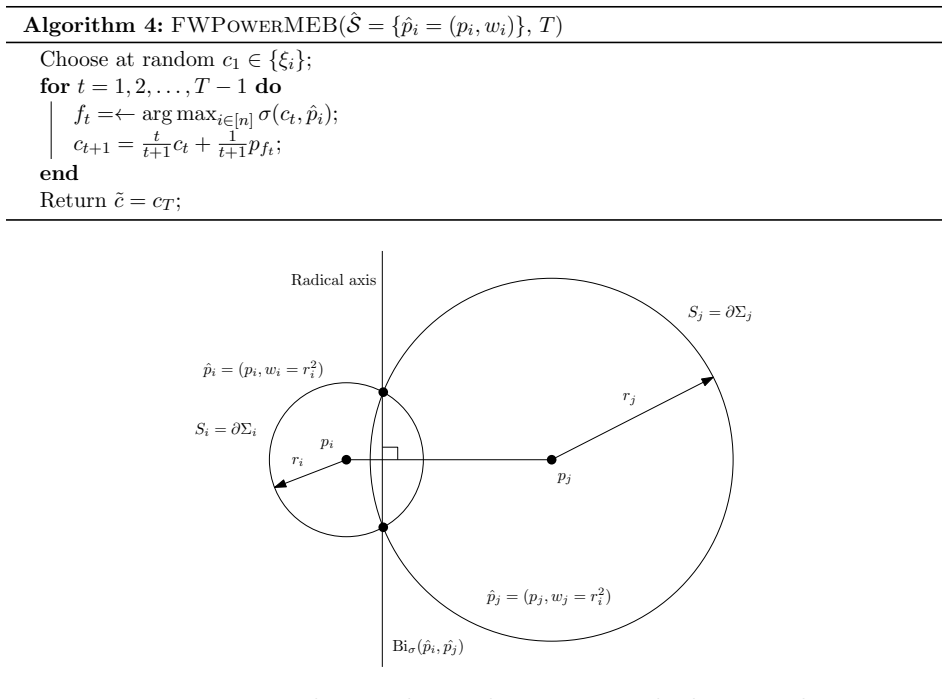
In this work, we revisit the problem of computing minimum enclosing Bregman balls (Bregman MEBs) of finite sets of parameters. First, we show that Bregman MEBs are equivalent to MEBs of corresponding weighted point sets with respect to the power distance. We then report an efficient Frank--Wolfe $(1+\epsilon)$-approximation algorithm for computing power MEBs, for any $\epsilon>0$. This power MEB approximation algorithm coincides with the Bregman MEB approximation algorithm of Nock and Nielsen (2005) when expressed in the dual gradient space. Finally, we show that the Bregman potential lifting transforms used to construct Bregman Voronoi diagrams can be reinterpreted as the classical paraboloid lifting transform applied to corresponding weighted point sets. In particular, Bregman MEB circumcenters lie on the farthest Bregman Voronoi diagrams or equivalently on the corresponding farthest power diagrams.