REVIEW 4 major objections 7 minor 13 references
A learned score correction turns unstable time steppers into schemes that stay on the manifold of admissible PDE states, with a stability bound independent of the number of steps.
Reviewed by Pith at T0; open to challenge. T0 means a machine referee read the full paper against a public rubric. the ladder, T0–T4 →
T0 review · grok-4.5
2026-07-31 00:44 UTC pith:YQZSL2H3
load-bearing objection Useful empirical stabilizer for fragile PDE steppers; the contraction theorem is clean on paper but never checked on the actual U-Nets. the 4 major comments →
Score-Based Stabilization for Time-Dependent Problems
The pith
A machine-rendered reading of the paper's core claim, the machinery that carries it, and where it could break.
Core claim
The score-based stabilization operator acts as a contraction toward the manifold of admissible states. When the provisional numerical update remains inside the score’s basin of attraction, the corrected two-stage scheme keeps the manifold distance bounded by a fixed ε for all time, independently of the number of steps (conditional manifold stability).
What carries the argument
The two-stage map: provisional update û = G_Δt(u) followed by the score correction S(û) = û + σ² s(û) (optionally composed with exact invariant projections). The score s ≈ ∇ log p is learned by denoising score matching on admissible snapshots; under an energy with PL inequality the correction is a uniform contraction onto the manifold.
Load-bearing premise
The learned score must behave like the gradient of an energy that contracts toward the admissible manifold on a whole neighborhood of that manifold; if the network fails to supply that contraction, the long-time bound collapses.
What would settle it
Train the U-Net score on the KdV or Burgers ensemble, then run the corrected leap-frog or FTCS scheme from an initial condition whose provisional steps systematically leave the claimed basin; if the manifold distance grows without bound or the solution still blows up while a classical stabilizer does not, the conditional-stability claim fails.
If this is right
- Inexpensive explicit or leap-frog integrators can be run at larger steps once a score corrector is trained, amortizing the offline cost over many simulations of the same PDE family.
- Classical artificial viscosity and spectral filters can be replaced or augmented by a learned correction that targets structure preservation rather than dissipation.
- When exact invariants (mass, L2, Hamiltonian) are known, combining score steps with projections yields both stability and machine-precision conservation.
- The same trained score transfers to unseen initial conditions of the same equation, so one model serves an entire ensemble rather than a single trajectory.
Where Pith is reading between the lines
- If the basin hypothesis can be checked cheaply online (e.g., by monitoring residual growth), the method could auto-reduce the step only when the provisional state leaves the basin, giving an adaptive hybrid of large and safe steps.
- The same contraction view suggests score correctors could stabilize other marginally stable discretizations (multisymplectic schemes, low-regularity integrators) without redesigning the spatial operator.
- Failure modes will likely appear first for solutions that leave the training measure—shocks stronger than those seen in PDEBench, or multi-soliton collisions far from the cosine training set—so coverage of the admissible manifold is the practical bottleneck.
Editorial analysis
A structured set of objections, weighed in public.
Referee Report
Summary. The manuscript proposes a two-stage stabilization framework for time-dependent PDEs in which a standard time-stepping update is followed by a learned score-based correction that drives the provisional state back toward the manifold of physically admissible states. The score is parameterized by a U-Net trained with denoising score matching on snapshots from high-fidelity solvers. Theoretically, the paper proves (i) that a Lipschitz correction with the manifold as fixed points preserves the integrator's order (Lemma A.1), (ii) a one-step distance bound for the provisional update (Lemma A.2), and (iii) that K gradient steps on an energy satisfying smoothness and Polyak–Łojasiewicz conditions contract toward the manifold (Lemma A.3), yielding a step-independent conditional stability result (Theorem 1 / A.1). Empirically, the method stabilizes otherwise-divergent baselines on advection (supercritical CFL), KdV (leap-frog blow-up at t≈2.34), NLS (amplitude/energy drift at large Δt), and Burgers (FTCS divergence), with an ablation study (Table 5), timestep-refinement control (Table 6), timing comparison (Table 7), and unseen-initial-condition generalization tests (Appendix G).
Significance. If the results hold, the paper makes a useful contribution at the interface of generative modeling and numerical analysis: it reframes stabilization as projection onto a learned admissible-state manifold, decoupling the stabilizer from hand-crafted, PDE-specific limiters. The experimental package is a genuine strength: four distinct PDEs, classical baselines (TVD, WENO-5, spectral filtering) at matched resolution, a component ablation isolating score vs. invariant-projection contributions, a refinement study showing the KdV baseline cannot be rescued by smaller Δt, and out-of-distribution initial-condition tests. The explicit remark in Appendix A distinguishing manifold stability from long-time trajectory accuracy is honest and appropriately scopes the claims. The paper is also well-positioned to be reproducible given the detail in Appendix H. The main weakness is that the theoretical headline (contraction, step-independent stability) is not connected to the deployed models: none of the constants or structural hypotheses of Lemma A.3 are verified, and the fixed-point assumption of Lemma A.1 is questionable for noise-smoothed learned scores. The empirical evidence for stabilization
major comments (4)
- [Appendix A, Lemma A.3 and Theorem A.1] The contraction result assumes (i) existence of an energy E with E=0 iff u∈M and quadratic bounds c±·dist², (ii) an L-Lipschitz gradient, and (iii) the PL inequality ‖∇E‖² ≥ 2μE on the sublevel set N. None of these is verified, or even estimated, for the deployed corrector R(x)=x+σ²s_θ(x) with s_θ a U-Net trained by DSM (Eqs. 15–17). Two distinct gaps follow. First, existence: s_θ is not architecturally constrained to be a gradient field (its Jacobian need not be symmetric), and DSM convergence in L2 to the true score does not imply the learned network is conservative; if s_θ has a nonzero rotational component, the energy E of Lemma A.3 does not exist and the proof's framing, not merely its constants, fails. Second, operational content: since μ, L, c±, and the basin radius are never measured, the key antecedent ρ_K(L_h ε + Ch^q) ≤ ε of Theorem A.1 cannot be checked for any experiment in
- [Appendix A, Lemma A.1 (fixed-point assumption)] Lemma A.1 assumes R(u)=u for all u∈M, i.e., the score vanishes on the admissible manifold. For a noise-smoothed density this holds only under symmetry/equilibrium conditions on the data distribution supported on M; with nonuniform training data on M (e.g., more snapshots of some solution profiles than others), the smoothed score generically has tangential components on M that advect states toward high-density regions. The corrector can then distort on-manifold dynamics even while 'stabilizing.' This is not hypothetical: the KdV results (Table 1) rely on exact invariant projections in addition to the score step, and the ablation (Table 5) shows the score-only variant drifts in I2 by 1.6e-3 while the projection eliminates drift. The authors should state the distributional condition under which R≈Id on M, discuss its dependence on training-data coverage, and clarify that the order-preservat
- [§5.2, Table 1] The KdV headline numbers conflate two messages. The score-corrected scheme reports err_pt = 0.42 at t=2 and 0.70 at t=10 — i.e., 42–70% relative pointwise error — while the text claims the corrected scheme 'accurately track[s] the slopes of the reference' and 'keeps pointwise errors low.' What the table actually supports is the (impressive) stability claim: the baseline diverges at t=2.34 while the corrected scheme integrates to t=10 with invariants at machine precision. The near-zero err_I2 and err_H are achieved by the exact invariant projections, not the score (Table 5: score-only err_pt 0.71 vs. full 0.70 — nearly identical pointwise error, with the projection supplying the invariant conservation). The claims in §5.2 and the conclusion should be reworded to attribute stability and invariant preservation to the correct components, and the qualitative-accuracy claim should be stated in
- [§5.4, Table 3] The divergence of TVD (Superbee) and WENO-5 on viscous Burgers at both Δt values is surprising and load-bearing for the comparison, since these are robust, widely used schemes for exactly this equation. Appendix C indicates the viscous term is treated explicitly in both baselines; at N=256 and Δt=4×10⁻³ the explicit viscous stability restriction (Δt ≲ Δx²/2ν) is plausibly violated, which would make the comparison one of time-integration choices rather than stabilization quality. The paper should state the PDEBench viscosity ν used, report the viscous and convective CFL numbers for each baseline, and justify that the classical baselines are run under conditions where they are expected to be stable (or acknowledge that the comparison is against explicitly-stabilized variants with the same restrictive time marching). As written, a reader cannot rule out that the baselines' failure is an imp
minor comments (7)
- [Appendix E] Typo: 'and thus enphisizetheadvantege of using the score correction scheme' — garbled sentence; also check the surrounding paragraph for OCR/formatting corruption.
- [Table 1] Column formatting appears corrupted: entries such as '6.120.78' and '8.220.91' run the err_H and err_pt columns together; 'errpt' for LF at t=2 (0.43) is reported under the wrong header alignment. Please re-typeset.
- [§4.1 / Appendix H] The role of the correction interval K is ambiguous: in Lemma A.3, K is the number of gradient steps composing R, while Appendix H's grid search over K∈{1,5,10,20} and the phrase 'correction interval' suggest K may instead be the stride between corrections. Please define K precisely and reconcile the two usages.
- [§5.3] Typo: 'we additionally provide a visualization of out method' → 'our method'. Also, Table 9 lists no enforced invariants for NLS, yet Table 2 reports very small Hamiltonian drift for the corrected scheme — a brief comment on why the score alone controls energy drift here (but not in KdV) would be informative.
- [§4.2 / inference] Training conditions on multiple noise levels σ (Eq. 15), but inference uses a single σ per experiment (App. H). Please clarify how the inference σ is chosen relative to the perturbation magnitude introduced by the provisional step, and whether the Tweedie interpretation (Eq. 9) is used to set it.
- [§5.1 / Appendix B.1] For advection, the training data are exact shifts of a small family of pulse profiles (App. H), so the learned manifold is essentially the orbit of the training profiles under translation. A short discussion of what the corrector can and cannot do for initial profiles outside this family (beyond the PDEBench ensemble) would strengthen the generalization discussion begun in Appendix G.
- [General] Notation is inconsistent between s(x) (analytic score, §3.2) and s_θ (learned score, §4.2); several statements in §4.5/Appendix A about 'the score' do not specify which is meant, though the distinction matters for the theory. Also, Theorem 1 in §4.5 refers to 'Lemma 3' — please align numbering with Appendix A (Lemma A.3).
Circularity Check
No algebraic circularity: conditional contraction theorem is self-contained under stated hypotheses; empirical claims are checked against external references, held-out ICs, and classical baselines.
full rationale
The paper’s load-bearing theoretical claim (Theorem 1 / Theorem A.1) is a standard conditional stability argument: if the provisional step stays in a basin where a gradient-based corrector contracts (Lemmas A.1–A.3: order preservation, one-step distance bound, PL/smooth energy descent), then manifold distance remains ≤ ε for all steps. The proof does not define the conclusion into the hypotheses, nor does it import a uniqueness theorem or ansatz from overlapping-author citations. The score model is trained by ordinary denoising score matching on high-fidelity snapshots; that makes the method dependent on an external oracle for the notion of “admissible,” but the paper does not then “predict” those same snapshots as a first-principles derivation—the evaluation is against independent spectral/PDEBench references, held-out initial conditions, and TVD/WENO/spectral-filter baselines (Tables 1–5, Figs. 2–10). Hyperparameters are grid-searched on held-out L2, which is ordinary tuning, not a fitted quantity renamed as a prediction of a closely related target. Exact invariant projections used for KdV make err_I2 = 0 by construction, but the paper’s ablation (Table 5) separates projection-only from score-only from the full method, and invariant conservation is not the central claimed derivation. Gaps between the PL/energy hypotheses and the deployed U-Net are correctness/verification issues, not circular reductions. Score 0 is therefore the proportionate finding.
Axiom & Free-Parameter Ledger
free parameters (4)
- correction noise level σ =
problem-dependent (e.g. 0.05 KdV/NLS, 0.1 Burgers, 0.05–0.2 advection)
- score step size η =
e.g. 3e-4 (KdV), 1e-3 (NLS), 0.01 (Burgers), 0.003–0.05 (advection)
- correction interval K =
1–20 depending on experiment
- U-Net depth/channels and training schedule =
see Tables 8–9 (0.18M–2.91M params)
axioms (5)
- domain assumption Physically admissible states concentrate on a manifold M that can be represented by a positive density p whose score is learnable by denoising score matching.
- standard math Tweedie’s formula: E[x|x̂] = x̂ + σ² ∇ log p(x̂) under Gaussian perturbation.
- ad hoc to paper On a sublevel set of an energy E with E=0 iff on M, ∇E is L-Lipschitz and satisfies the PL inequality ∥∇E∥² ≥ 2μE, so K gradient steps contract distance to M.
- ad hoc to paper Whenever the constraint residual r_j ≤ ε, the provisional predictor lands inside the score’s basin and obeys the one-step distance bound r̂ ≤ L_h ε + C h^q.
- domain assumption Exact discrete projections can enforce selected invariants (mass, L2, Hamiltonian) after the score step without destroying the contraction picture.
invented entities (1)
-
Score-based stabilization operator S (single or multi-step score correction, optionally composed with invariant projections)
no independent evidence
read the original abstract
We propose a score-based stabilization framework for numerical simulation of partial differential equations, in which a learned score model defines a stabilization operator applied to provisional numerical updates. This operator augments standard time-stepping schemes by enforcing structure and physical consistency through a correction that drives iterates toward the manifold of admissible states. We show that the stabilization operator acts as a contraction toward this manifold, yielding a correction mechanism with basin-conditional stability. Numerical experiments on Advection, Korteweg-de Vries (KdV), Nonlinear Schrodinger (NLS), and Burgers' equations demonstrate improved robustness, suppression of nonphysical instabilities, and preservation of qualitative dynamics.
Figures


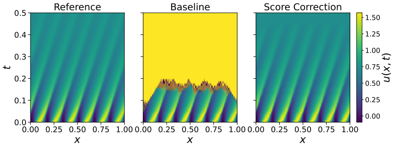

Reference graph
Works this paper leans on
-
[5]
Advection using PDEBenchWe use to the advection problem introduced in Section 5.1, using the version of this problem supplied by PDEBench (Takamoto et al. 2022). For the evaluation, we fix the domain lengthL= 1, the advection speeda= 1, and integrate to a final timeT= 2, corresponding to two complete domain traversals. Initial conditionsu0(x)are drawn fro...
2022
-
[8]
Miyatake, Y.; Irie, K.; and Matsuda, T
Sdedit: Guided image synthesis and editing with stochastic differential equations.arXiv preprint arXiv:2108.01073. Miyatake, Y.; Irie, K.; and Matsuda, T
-
[9]
InInterna- tional Conference on Learning Representations
Score-Based Generative Mod- eling through Stochastic Differential Equations. InInterna- tional Conference on Learning Representations. Sulem,C.;andSulem,P.-L.2007.ThenonlinearSchrödinger equation: self-focusing and wave collapse, volume
2007
-
[12]
All experiments were conducted using NVIDIA GeForce RTX 4090 GPUs. For hyperparameter selection, the noise levelσ, the step sizeη, and the correction intervalKwere chosen by grid search overσ∈ {0.02,0.05,0.1,0.2,0.3,0.5,0.8},η∈ {10−5,10 −4,3×10 −4,10 −3,3×10 −3,10 −2,3×10 −2}, andK∈ {1,5,10,20}. The configuration minimizing the relative L2 error on the he...
2048
-
[1614]
2012.Geometric Numerical Integration and Schrödinger Equations
Faou, E. 2012.Geometric Numerical Integration and Schrödinger Equations. European Mathematical Society. Zurich Lectures in Advanced Mathematics. Godunov,S.K.1959. Adifferenceschemefornumericalso- lutionofdiscontinuoussolutionofhydrodynamicequations. Math. Sbornik, 47: 271–306. Gottlieb,D.;andHesthaven,J.S.2001. Spectralmethodsfor hyperbolicproblems.Journa...
2012
-
[1996]
Efficient implementa- tion of weighted ENO schemes.Journal of computational physics, 126(1): 202–228. Kingma,D.P.;andBa,J.2014. Adam:Amethodforstochas- tic optimization.arXiv preprint arXiv:1412.6980. Kochkov, D.; Smith, J. A.; Alieva, A.; Wang, Q.; Brenner, M. P.; and Hoyer, S
Pith/arXiv arXiv 2014
-
[2005]
Bar-Sinai,Y.;Hoyer,S.;Hickey,J.;andBrenner,M.P.2019
On symplectic andmultisymplecticschemesfortheKdVequation.Journal of Scientific Computing, 25(1–2): 83–104. Bar-Sinai,Y.;Hoyer,S.;Hickey,J.;andBrenner,M.P.2019. Learning data-driven discretizations for partial differential equations.ProceedingsoftheNationalAcademyofSciences, 116(31): 15344–15349. Boris,J.P.;andBook,D.L.1973. Flux-correctedtransport. I. SHA...
2019
-
[2008]
Comp., 77: 2141–2153
On splitting methods for Schrödinger- Poisson and cubic nonlinear Schrödinger equations.Math. Comp., 77: 2141–2153. Luo,S.;andHu,W.2021.Score-basedpointclouddenoising. InProceedingsoftheIEEE/CVFinternationalconferenceon computer vision, 4583–4592. MacCormack, R. W
2021
-
[2014]
The KdV and NLS errors are computed against high-accuracy spectral reference solutions
Learning rate2×10 −4 2×10⁻⁴ 2×10⁻⁴ 2×10⁻⁴ LR schedule Cosine Cosine Cosine Cosine Batch size512 512 512 512 Epochs500 500 500 500 Training-data resolution2048 2048 2048 1024 Training-data∆tExact Exact Exact Exact Correction (inference) σ0.1 0.05 0.2 0.05 Stepη0.003 0.03 0.05 0.003 IntervalK5 10 20 10 Enforced invariants None Clamp[0,1]Clamp+Mass Mass+L 2 ...
2048
-
[2020]
Hyvärinen,A.2005
Denoising diffusion probabilistic models.Advances in neural information pro- cessing systems, 33: 6840–6851. Hyvärinen,A.2005. EstimationofNon-NormalizedStatisti- calModelsbyScoreMatching.JournalofMachineLearning Research, 6: 695–709. Jiang, G.-S.; and Shu, C.-W
2005
-
[2021]
Machine learning–accelerated computational fluid dynamics.Proceedings of the National Academy of Sciences, 118(21): e2101784118. Lax, P. D. 1973.Hyperbolic systems of conservation laws and the mathematical theory of shock waves. SIAM. LeVeque, R. 1990.Numerical Methods for Conservation Laws. Birkhauser. LeVeque, R. J. 2002.Finite volume methods for hyperb...
1973
-
[2022]
Efron,B.2011
Riemannian score-based generative modelling.Advances in neural information pro- cessing systems, 35: 2406–2422. Efron,B.2011. Tweedie’sFormulaandSelectionBias.Jour- naloftheAmericanStatisticalAssociation,106(496):1602–
2011
-
[2025]
VonNeumann, J.; and Richtmyer, R
Joint Bayesian Inference of Parameter and Discretization Error Uncertainties in ODE Models.arXiv preprint arXiv:2511.23010. VonNeumann, J.; and Richtmyer, R. D
discussion (0)
Sign in with ORCID, Apple, or X to comment. Anyone can read and Pith papers without signing in.