REVIEW 3 major objections 4 minor 91 references
SYNTHESIZER now integrates photoionised gas emission into synthetic galaxy spectra
Reviewed by Pith at T0; open to challenge. T0 means a machine referee read the full paper against a public rubric. the ladder, T0–T4 →
T0 review · deepseek-v4-flash
2026-08-01 07:24 UTC pith:WG5E5MHJ
load-bearing objection Solid, useful software paper; the single-zone Cloudy-per-particle mapping is a real limitation but exactly the kind of thing a referee can push on without sinking the paper. the 3 major comments →
Stellar photoionisation modelling in SYNTHESIZER
The pith
A machine-rendered reading of the paper's core claim, the machinery that carries it, and where it could break.
Core claim
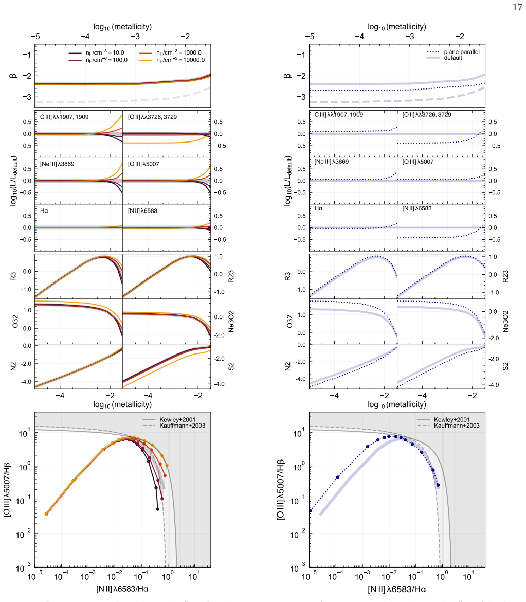
The central claim is that SYNTHESIZER provides a flexible, physically motivated framework for modelling stellar and nebular emissions, serving as a vital link between theory and observations. The paper argues that processing simple stellar population spectra through Cloudy with a carefully chosen default configuration—spherical geometry with inner radius 0.01 pc, a reference ionisation parameter that scales with the cube root of the ionising photon rate, gas-phase metallicity matching the stellar metallicity, Jenkins (2009) depletion with F*=0.5, and Orion-type grains—yields reliable predictions across a wide range of ages, metallicities, and galaxy types. The parameter exploration quantifie
What carries the argument
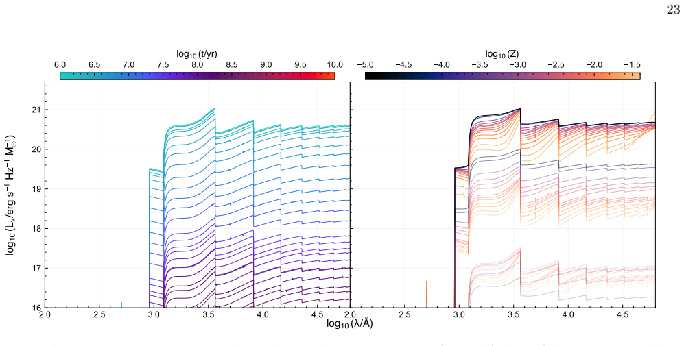
The central machinery is the pre-computed spectral grid: each simple stellar population (SSP) from a stellar population synthesis model, such as BPASS, is run through the Cloudy photoionisation code to store incident, transmitted, and nebular spectra plus line luminosities. The key identity is the reference ionisation parameter scaling, US = (QH/QH,ref)^(1/3) Uref, which sets the ionisation parameter for each grid point in spherical geometry based on the ionising photon production rate relative to a reference SSP at t=1 Myr and Z=0.01. This avoids imposing an artificial geometry evolution when age or metallicity changes.
Load-bearing premise
The load-bearing premise is that each star particle's unresolved gas can be represented by a single spherical Cloudy HII-region model whose gas-phase metallicity equals the stellar metallicity.
What would settle it
A comparison with resolved HII regions in the local Universe where both the ionising stellar population and the gas-phase abundances are measured: if the observed line ratios deviate systematically from the model grid by more than the grid's sensitivity range, the equal-metallicity or single-geometry assumptions would be falsified.
If this is right
- Synthetic spectra from cosmological simulations will now include physically motivated nebular lines and continua, enabling direct comparison with JWST, Euclid, and future ELT spectroscopy.
- The framework can be used to calibrate dust attenuation prescriptions by matching predicted Hα luminosity functions to observed ones.
- The sensitivity maps show which parameters (e.g., depletion, grain mixture) must be constrained before line-ratio diagnostics can be trusted for metallicity or ionisation parameter inference.
- The reference ionisation parameter scaling makes predictions robust to SPS model choice for line ratios, while absolute line luminosities remain sensitive to the ionising photon budget.
- The package's flexibility means the same grids can be used for SED fitting and forward modelling, unifying interpretation and prediction.
Where Pith is reading between the lines
- A natural extension would be to replace the single-zone Cloudy model with a distribution of ionisation parameters or escape fractions per star particle, which could be tested against resolved HII region observations.
- The strong sensitivity of the BPT diagram's high-metallicity locus to dust depletion suggests that metallicity calibrations derived without dust-depletion corrections could be systematically biased, a caution that applies beyond this package.
- Coupling the grids to a machine-learning emulator, as the authors note is underway, could make full photoionisation models tractable in Bayesian parameter estimation and simulation-based inference.
- One could test the equal-metallicity assumption by applying the package to galaxies with independently measured stellar and gas-phase metallicities from stacked spectra.
Editorial analysis
A structured set of objections, weighed in public.
Referee Report
Summary. The paper presents the implementation of photoionised gas emission in the SYNTHESIZER package, using Cloudy to process stellar population grids and produce nebular line and continuum predictions. It describes the default modelling assumptions (reference ionisation parameter, spherical geometry, constant density, gas-phase metallicity tied to the SSP, depletion and grain prescriptions, ionisation-bounded stopping) and systematically explores the sensitivity of UV continuum slopes, emission-line luminosities, and diagnostic ratios to SPS model, IMF, ionisation parameter, density, abundance pattern, depletion, and dust. Example applications include a parametric galaxy, a single TNG50 galaxy, and the full EAGLE simulation, where Hα luminosity functions and equivalent width distributions are compared to observational data. The authors claim that SYNTHESIZER provides a flexible, physically motivated framework for modelling stellar and nebular emission.
Significance. If the central claim is borne out, this is a valuable open-source contribution: the code and pre-computed grids are publicly available with version-stamped releases, and the systematic parameter exploration provides a useful baseline for interpreting synthetic observations. The range of applications—from toy models to cosmological simulations—demonstrates genuine versatility. However, the validation is limited and partially circular: the single observational check of the Hα luminosity function uses a dust attenuation prescription calibrated with the same BPASS v2.2.1 SPS model, and the per-particle single-zone HII-region mapping is not directly tested. The paper is transparent about several acknowledged approximations (Z_gas=Z_SSP, grain scheme self-consistency), which is commendable but does not remove the need for robustness tests.
major comments (3)
- [§5.6, §3.1.2, §3.3] The default mapping of every star particle to a single constant-density spherical Cloudy HII region (n_H=10^2.5 cm^-3, R0=0.01 pc, Z_gas=Z_SSP, and the cube-root ionisation-parameter scaling of Eq. 4) is a strong idealisation when applied to cosmological simulation particles. The paper does not test this mapping against the resolved gas distribution in EAGLE or TNG50, nor does it quantify how varying n_H, U_ref, or the stopping column would affect the predicted Hα luminosity function. The EAGLE Hα LF and the equivalent-width distributions are central demonstrations, so a robustness test with plausible alternative mappings or an explicit estimate of the systematic uncertainty is needed to support the claim that the tool 'correctly predicts nebular line and continuum emission.'
- [§5.6] The agreement of the default-model Hα LF at z=2.237 with Sobral et al. (2013) is partly circular for the validation of the photoionisation modelling: the FLARES dust attenuation prescription was calibrated using the same BPASS v2.2.1 SPS model to match the z=5 UVLF (Vijayan et al. 2021), as acknowledged in the text. The agreement can therefore be driven largely by the dust calibration and SPS choice rather than by the photoionisation modelling itself. The authors should either compare intrinsic (dust-free) Hα LFs, use an independently calibrated dust prescription, or vary the SPS model with a fixed dust prescription to isolate the photoionisation contribution. The current figure cannot distinguish between these degeneracies.
- [§3.3, §3.3.4] The default assumption that the gas-phase metallicity equals the SSP metallicity is explicitly acknowledged as 'may not be fully self-consistent,' and the depletion-to-grain implementation is likewise stated to be 'not fully self-consistent.' These assumptions underlie every grid and every application in the paper. The parameter exploration in Section 4 varies the metallicity of the stellar population and the gas simultaneously, so it does not isolate the effect of decoupling Z_gas from Z_SSP. A quantitative test of this approximation—e.g., a small grid with Z_gas offset from Z_SSP, or a discussion of the expected bias from abundance decoupling—would materially strengthen the claim that the framework is physically motivated and would help users assess the default grids.
minor comments (4)
- [Data Availability] The data availability statement says that all scripts to generate the plots 'will be made publicly available on Github on the acceptance of the paper.' For a software-centric paper, releasing plot scripts at submission would aid reproducibility and reviewer verification.
- [§3.4] The discussion of the stopping criterion notes that ionisation-bounded models with dust produce attenuation that depends on the ionising photon rate, but the quantitative effect on the EAGLE Hα LF (e.g., comparing to a fixed column-density stop) is not shown. A brief figure or table would clarify the impact of this modelling choice.
- [Fig. 29] The visual agreement with Sobral et al. (2013) and Khostovan et al. (2024) would be easier to assess with residuals or a reduced chi-square statistic; for the luminosity function, plotting the observed error bars and model uncertainties would also help.
- [Throughout] Minor typographical and formatting issues: 'Hiiregions' appears without proper spacing in several places; the caption of Fig. 23 says 'The same as Figure 21 but showing the resulting nebular continuum spectra' but the axes are identical to Fig. 21—consider clarifying the difference.
Circularity Check
No significant circularity: the paper is a forward-modeling software description; no target observable is fitted to produce the central predictions.
full rationale
The paper's central claims are demonstrations that a grid of SPS spectra processed through the external photoionisation code Cloudy yields nebular line/continuum predictions and a parameter-dependence map. No observable is used to fit the model parameters: U_ref=0.01, n_H=10^2.5, the Galactic Concordance abundance pattern, Jenkins F*=0.5 depletion, and the ionisation-bounded stopping criterion are all disclosed modelling choices, not fits to data. Equation (4) is a scaling convention for the ionisation parameter, not an inverse derivation from a target observable. The EAGLE H-alpha luminosity function comparison uses the FLARES dust attenuation model from Vijayan et al. (2021), which was calibrated to the external z=5 UVLF (Bouwens et al. 2015); the H-alpha LF at z=2.237 is a different observable and is not the calibration target, so the comparison is not forced by construction. Self-citations to Lovell et al. (2025a), Roper et al. (2026), and Vijayan et al. (2021) provide code and dust-model provenance rather than a load-bearing uniqueness argument. The paper explicitly flags its own limitations (e.g., gas-phase metallicity equal to SSP metallicity 'may not be fully self-consistent'; the stopping criterion affects attenuation), but acknowledged modelling limitations are not circularity. No 'prediction' reduces to an input by definition.
Axiom & Free-Parameter Ledger
free parameters (8)
- Reference ionisation parameter U_ref =
0.01
- Hydrogen density n_H =
10^2.5 cm^-3
- Jenkins depletion scale F_star =
0.5
- Ionising photon escape fraction f_esc =
0.3 (toy example; user-specified)
- Lyman-alpha escape fraction f_Ly-alpha,esc =
user-specified
- Stopping electron fraction =
0.01
- Inner radius R0 for spherical geometry =
0.01 pc
- Dust attenuation normalisation (Flares prescription) =
calibrated to z=5 UVLF (Bouwens+2015) with BPASS v2.2.1 in Vijayan+2021
axioms (6)
- domain assumption Cloudy C23.01 accurately predicts photoionised gas emission for a given incident SED and gas model.
- domain assumption Default SPS model (BPASS v2.2.1, Chabrier IMF, 0.1-300 Msun) is a faithful representation of young stellar populations and their ionising photon production.
- ad hoc to paper The reference ionisation-parameter scaling US = (QH/QH,ref)^{1/3} U_ref (Eq. 4) is a physically appropriate way to model HII regions around evolving stellar populations.
- domain assumption Gas-phase metallicity (including depletion) equals the SSP metallicity.
- domain assumption Ionisation-bounded stopping criterion (electron fraction < 0.01) is appropriate; escaping photons handled separately via f_esc.
- ad hoc to paper Dust grains can be represented by Orion/ISM mixtures plus PAHs, with scales set by carbon and silicon depletion.
read the original abstract
Emission from photoionised gas surrounding young stellar populations ($H\text{II}$ regions) provides critical diagnostics of the physical conditions in star forming galaxies. This emission constrains the gas properties, the nature of ionising sources, and generates essential features for determining galaxy redshifts. To leverage spectroscopic observations to test galaxy formation models, it is essential to incorporate these emissions into synthetic datasets. Here, we present the integration of photoionised gas emission into the SYNTHESIZER package (https://synthesizer-project.github.io) and demonstrate its application. We quantify the impact of key modelling assumptions - including stellar population synthesis models, initial mass functions, ionisation parameter, gas density, geometry, abundance pattern, elemental depletion, and dust - on spectral diagnostics. Furthermore, we demonstrate the versatility of SYNTHESIZER through its application in different scenarios ranging from exploring emission in toy parametric models to large-volume cosmological simulations with realistic star formation and metal enrichment histories. Taken together, SYNTHESIZER provides a flexible, physically motivated framework to model stellar and nebular emissions, serving as a vital link between theory and observations in the era of next-generation spectroscopic missions.
Figures






Reference graph
Works this paper leans on
-
[1]
Abel N. P., van Hoof P. A. M., Shaw G., Ferland G. J., Elwert T., 2008, @doi [ ] 10.1086/591505 , https://ui.adsabs.harvard.edu/abs/2008ApJ...686.1125A 686, 1125
doi:10.1086/591505 2008
-
[2]
Allen M. G., Groves B. A., Dopita M. A., Sutherland R. S., Kewley L. J., 2008, @doi [ ] 10.1086/589652 , https://ui.adsabs.harvard.edu/abs/2008ApJS..178...20A 178, 20
doi:10.1086/589652 2008
-
[3]
Anders P., Fritze-v. Alvensleben U., 2003, @doi [ ] 10.1051/0004-6361:20030151 , https://ui.adsabs.harvard.edu/abs/2003A&A...401.1063A 401, 1063
-
[4]
Arjona-G \'a lvez E., Di Cintio A., Grand R. J. J., Sales L. V., Canalizo G., Matamoro Zatarain T., Vijayan A. P., 2026, @doi [arXiv e-prints] 10.48550/arXiv.2606.30726 , https://ui.adsabs.harvard.edu/abs/2026arXiv260630726A p. arXiv:2606.30726
work page internal anchor Pith review Pith/arXiv arXiv doi:10.48550/arxiv.2606.30726 2026
-
[5]
Arrabal Haro P., et al., 2023, @doi [ ] 10.1038/s41586-023-06521-7 , https://ui.adsabs.harvard.edu/abs/2023Natur.622..707A 622, 707
-
[6]
Asplund M., Grevesse N., Sauval A. J., Scott P., 2009, @doi [ ] 10.1146/annurev.astro.46.060407.145222 , https://ui.adsabs.harvard.edu/abs/2009ARA&A..47..481A 47, 481
arXiv 2009
-
[7]
Astropy Collaboration et al., 2013, @doi [ ] 10.1051/0004-6361/201322068 , http://adsabs.harvard.edu/abs/2013A
-
[8]
Astropy Collaboration et al., 2018, @doi [ ] 10.3847/1538-3881/aabc4f , https://ui.adsabs.harvard.edu/abs/2018AJ....156..123A 156, 123
-
[9]
Astropy Collaboration et al., 2022, @doi [ ] 10.3847/1538-4357/ac7c74 , https://ui.adsabs.harvard.edu/abs/2022ApJ...935..167A 935, 167
-
[10]
Barrow K. S. S., Wise J. H., Norman M. L., O'Shea B. W., Xu H., 2017, @doi [ ] 10.1093/mnras/stx1181 , https://ui.adsabs.harvard.edu/abs/2017MNRAS.469.4863B 469, 4863
-
[11]
Baugh C. M., Lacey C. G., Gonzalez-Perez V., Manzoni G., 2022, @doi [ ] 10.1093/mnras/stab3506 , https://ui.adsabs.harvard.edu/abs/2022MNRAS.510.1880B 510, 1880
-
[12]
Begley R., et al., 2026, @doi [ ] 10.1093/mnras/staf1995 , https://ui.adsabs.harvard.edu/abs/2026MNRAS.545f1995B 545, staf1995
-
[13]
Boquien M., Burgarella D., Roehlly Y., Buat V., Ciesla L., Corre D., Inoue A. K., Salas H., 2019, @doi [ ] 10.1051/0004-6361/201834156 , https://ui.adsabs.harvard.edu/abs/2019A&A...622A.103B 622, A103
-
[14]
Bouwens R. J., et al., 2015, @doi [ ] 10.1088/0004-637X/803/1/34 , https://ui.adsabs.harvard.edu/abs/2015ApJ...803...34B 803, 34
-
[15]
Bruzual G., Charlot S., 2003, @doi [ ] 10.1046/j.1365-8711.2003.06897.x , https://ui.adsabs.harvard.edu/abs/2003MNRAS.344.1000B 344, 1000
arXiv 2003
-
[16]
Bruzual A. G., Charlot S., 1993, @doi [ ] 10.1086/172385 , https://ui.adsabs.harvard.edu/abs/1993ApJ...405..538B 405, 538
doi:10.1086/172385 1993
-
[17]
Byler N., Dalcanton J. J., Conroy C., Johnson B. D., 2017, @doi [ ] 10.3847/1538-4357/aa6c66 , https://ui.adsabs.harvard.edu/abs/2017ApJ...840...44B 840, 44
-
[18]
Byrne C. M., Eldridge J. J., Stanway E. R., 2025, @doi [ ] 10.1093/mnras/staf178 , https://ui.adsabs.harvard.edu/abs/2025MNRAS.537.2433B 537, 2433
-
[19]
Carnall A. C., McLure R. J., Dunlop J. S., Dav \'e R., 2018, @doi [ ] 10.1093/mnras/sty2169 , https://ui.adsabs.harvard.edu/abs/2018MNRAS.480.4379C 480, 4379
-
[20]
Ceverino D., Klessen R. S., Glover S. C. O., 2019, @doi [ ] 10.1093/mnras/stz079 , https://ui.adsabs.harvard.edu/abs/2019MNRAS.484.1366C 484, 1366
-
[21]
Chabrier G., 2003, @doi [ ] 10.1086/376392 , 115, 763
doi:10.1086/376392 2003
-
[22]
Chaikin E., et al., 2026, @doi [ ] 10.1093/mnras/stag300 , https://ui.adsabs.harvard.edu/abs/2026MNRAS.548ag300C 548, stag300
-
[23]
M., 2000, @doi [ ] 10.1086/309250 , https://ui.adsabs.harvard.edu/abs/2000ApJ...539..718C 539, 718
Charlot S., Fall S. M., 2000, @doi [ ] 10.1086/309250 , https://ui.adsabs.harvard.edu/abs/2000ApJ...539..718C 539, 718
doi:10.1086/309250 2000
-
[25]
Chatzikos M., et al., 2023, @doi [ ] 10.22201/ia.01851101p.2023.59.02.12 , https://ui.adsabs.harvard.edu/abs/2023RMxAA..59..327C 59, 327
-
[27]
Conroy C., Gunn J. E., White M., 2009, @doi [ ] 10.1088/0004-637X/699/1/486 , https://ui.adsabs.harvard.edu/abs/2009ApJ...699..486C 699, 486
-
[28]
A., et al., 2015, @doi [ ] 10.1093/mnras/stv725 , 450, 1937
Crain R. A., et al., 2015, @doi [ ] 10.1093/mnras/stv725 , 450, 1937
-
[29]
Dopita M. A., et al., 2006, @doi [ ] 10.1086/508261 , https://ui.adsabs.harvard.edu/abs/2006ApJS..167..177D 167, 177
doi:10.1086/508261 2006
-
[30]
T., 2011, Physics of the Interstellar and Intergalactic Medium
Draine B. T., 2011, Physics of the Interstellar and Intergalactic Medium
2011
-
[31]
Eldridge J. J., Stanway E. R., 2009, @doi [ ] 10.1111/j.1365-2966.2009.15514.x , https://ui.adsabs.harvard.edu/abs/2009MNRAS.400.1019E 400, 1019
arXiv 2009
-
[32]
Feltre A., Charlot S., Gutkin J., 2016, @doi [ ] 10.1093/mnras/stv2794 , https://ui.adsabs.harvard.edu/abs/2016MNRAS.456.3354F 456, 3354
-
[33]
Ferland G. J., Korista K. T., Verner D. A., Ferguson J. W., Kingdon J. B., Verner E. M., 1998, @doi [ ] 10.1086/316190 , https://ui.adsabs.harvard.edu/abs/1998PASP..110..761F 110, 761
doi:10.1086/316190 1998
-
[34]
Ferland G. J., et al., 2013, @doi [ ] 10.48550/arXiv.1302.4485 , https://ui.adsabs.harvard.edu/abs/2013RMxAA..49..137F 49, 137
-
[35]
Ferland G. J., et al., 2017, @doi [ ] 10.48550/arXiv.1705.10877 , https://ui.adsabs.harvard.edu/abs/2017RMxAA..53..385F 53, 385
-
[36]
Garg P., et al., 2022, @doi [ ] 10.3847/1538-4357/ac43b8 , https://ui.adsabs.harvard.edu/abs/2022ApJ...926...80G 926, 80
-
[37]
Groves B. A., Dopita M. A., Sutherland R. S., 2004, @doi [ ] 10.1086/421113 , https://ui.adsabs.harvard.edu/abs/2004ApJS..153....9G 153, 9
doi:10.1086/421113 2004
-
[38]
Gunasekera C. M., Ji X., Chatzikos M., Yan R., Ferland G., 2022, @doi [ ] 10.1093/mnras/stac022 , https://ui.adsabs.harvard.edu/abs/2022MNRAS.512.2310G 512, 2310
-
[39]
Gunasekera C. M., van Hoof P. A. M., Chatzikos M., Ferland G. J., 2023, @doi [Research Notes of the American Astronomical Society] 10.3847/2515-5172/ad0e75 , https://ui.adsabs.harvard.edu/abs/2023RNAAS...7..246G 7, 246
-
[40]
Gutkin J., Charlot S., Bruzual G., 2016, @doi [ ] 10.1093/mnras/stw1716 , https://ui.adsabs.harvard.edu/abs/2016MNRAS.462.1757G 462, 1757
-
[41]
R., et al., 2020, @doi [Nature] 10.1038/s41586-020-2649-2 , 585, 357
Harris C. R., et al., 2020, @doi [Nature] 10.1038/s41586-020-2649-2 , 585, 357
-
[42]
Harvey T., et al., 2026, @doi [ ] 10.1093/mnras/stag282 , https://ui.adsabs.harvard.edu/abs/2026MNRAS.547ag282H 547, stag282
-
[43]
Hirschmann M., Charlot S., Feltre A., Naab T., Choi E., Ostriker J. P., Somerville R. S., 2017, @doi [ ] 10.1093/mnras/stx2180 , https://ui.adsabs.harvard.edu/abs/2017MNRAS.472.2468H 472, 2468
-
[44]
Hirschmann M., Charlot S., Feltre A., Naab T., Somerville R. S., Choi E., 2019, @doi [ ] 10.1093/mnras/stz1256 , https://ui.adsabs.harvard.edu/abs/2019MNRAS.487..333H 487, 333
-
[45]
Hirschmann M., et al., 2023, @doi [MNRAS] 10.1093/mnras/stad2955 , 526, 3610
-
[46]
D., 2007, @doi [Computing in Science & Engineering] 10.1109/MCSE.2007.55 , 9, 90
Hunter J. D., 2007, @doi [Computing in Science & Engineering] 10.1109/MCSE.2007.55 , 9, 90
-
[47]
Indriolo N., Geballe T. R., Oka T., McCall B. J., 2007, @doi [ ] 10.1086/523036 , https://ui.adsabs.harvard.edu/abs/2007ApJ...671.1736I 671, 1736
doi:10.1086/523036 2007
-
[48]
Jenkins E. B., 2009, @doi [ ] 10.1088/0004-637X/700/2/1299 , https://ui.adsabs.harvard.edu/abs/2009ApJ...700.1299J 700, 1299
-
[49]
Jin Y., Kewley L. J., Sutherland R., 2022, @doi [ ] 10.3847/1538-4357/ac48f3 , https://ui.adsabs.harvard.edu/abs/2022ApJ...927...37J 927, 37
-
[50]
D., Leja J., Conroy C., Speagle J
Johnson B. D., Leja J., Conroy C., Speagle J. S., 2021, @doi [ ] 10.3847/1538-4365/abef67 , https://ui.adsabs.harvard.edu/abs/2021ApJS..254...22J 254, 22
-
[51]
Katz H., et al., 2023, @doi [The Open Journal of Astrophysics] 10.21105/astro.2309.03269 , https://ui.adsabs.harvard.edu/abs/2023OJAp....6E..44K 6, 44
Pith/arXiv arXiv 2023
-
[52]
Kauffmann G., et al., 2003, @doi [ ] 10.1111/j.1365-2966.2003.07154.x , https://ui.adsabs.harvard.edu/abs/2003MNRAS.346.1055K 346, 1055
arXiv 2003
-
[53]
Kewley L. J., Dopita M. A., Sutherland R. S., Heisler C. A., Trevena J., 2001, @doi [ ] 10.1086/321545 , https://ui.adsabs.harvard.edu/abs/2001ApJ...556..121K 556, 121
doi:10.1086/321545 2001
-
[54]
Kewley L. J., Nicholls D. C., Sutherland R. S., 2019, @doi [ ] 10.1146/annurev-astro-081817-051832 , https://ui.adsabs.harvard.edu/abs/2019ARA&A..57..511K 57, 511
-
[55]
Khostovan A. A., Malhotra S., Rhoads J. E., Sobral D., Harish S., Tilvi V., Coughlin A., Rezaee S., 2024, @doi [ ] 10.1093/mnras/stae2395 , https://ui.adsabs.harvard.edu/abs/2024MNRAS.535.2903K 535, 2903
-
[56]
Kroupa P., 2001, @doi [ ] 10.1046/j.1365-8711.2001.04022.x , https://ui.adsabs.harvard.edu/abs/2001MNRAS.322..231K 322, 231
arXiv 2001
-
[57]
Llerena M., et al., 2026, @doi [ ] 10.1051/0004-6361/202557897 , https://ui.adsabs.harvard.edu/abs/2026A&A...708A.152L 708, A152
-
[58]
Lovell C. C., Vijayan A. P., Thomas P. A., Wilkins S. M., Barnes D. J., Irodotou D., Roper W., 2021, @doi [ ] 10.1093/mnras/staa3360 , https://ui.adsabs.harvard.edu/abs/2021MNRAS.500.2127L 500, 2127
-
[59]
Lovell C. C., Roper W. J., Vijayan A. P., Wilkins S. M., Newman S., Seeyave L., 2025a, @doi [The Open Journal of Astrophysics] 10.33232/001c.145766 , https://ui.adsabs.harvard.edu/abs/2025OJAp....8E.152L 8, 152
-
[60]
Lovell C. C., et al., 2025b, @doi [ ] 10.1093/mnras/staf1888 , https://ui.adsabs.harvard.edu/abs/2025MNRAS.544.3949L 544, 3949
-
[61]
Madau P., Dickinson M., 2014, @doi [ ] 10.1146/annurev-astro-081811-125615 , https://ui.adsabs.harvard.edu/abs/2014ARA&A..52..415M 52, 415
-
[62]
Maraston C., 1998, @doi [ ] 10.1046/j.1365-8711.1998.01947.x , https://ui.adsabs.harvard.edu/abs/1998MNRAS.300..872M 300, 872
arXiv 1998
-
[63]
Maraston C., 2005, @doi [ ] 10.1111/j.1365-2966.2005.09270.x , https://ui.adsabs.harvard.edu/abs/2005MNRAS.362..799M 362, 799
arXiv 2005
-
[64]
Maraston C., Str \"o mb \"a ck G., 2011, @doi [ ] 10.1111/j.1365-2966.2011.19738.x , https://ui.adsabs.harvard.edu/abs/2011MNRAS.418.2785M 418, 2785
arXiv 2011
-
[65]
Maraston C., et al., 2020, @doi [ ] 10.1093/mnras/staa1489 , https://ui.adsabs.harvard.edu/abs/2020MNRAS.496.2962M 496, 2962
-
[66]
Mathis J. S., Rumpl W., Nordsieck K. H., 1977, @doi [ ] 10.1086/155591 , https://ui.adsabs.harvard.edu/abs/1977ApJ...217..425M 217, 425
doi:10.1086/155591 1977
-
[67]
Nelson D., et al., 2019, @doi [ ] 10.1093/mnras/stz2306 , https://ui.adsabs.harvard.edu/abs/2019MNRAS.490.3234N 490, 3234
-
[68]
Newman S. L., Lovell C. C., Maraston C., Roper W. J., Vijayan A. P., Wilkins S. M., Giavalisco M., Saxena A., 2026, @doi [ ] 10.1093/mnras/staf1866 , https://ui.adsabs.harvard.edu/abs/2026MNRAS.545f1866N 545, staf1866
-
[69]
Nicholls D. C., Sutherland R. S., Dopita M. A., Kewley L. J., Groves B. A., 2017, @doi [ ] 10.1093/mnras/stw3235 , https://ui.adsabs.harvard.edu/abs/2017MNRAS.466.4403N 466, 4403
-
[70]
Orsi \'A ., Padilla N., Groves B., Cora S., Tecce T., Gargiulo I., Ruiz A., 2014, @doi [ ] 10.1093/mnras/stu1203 , https://ui.adsabs.harvard.edu/abs/2014MNRAS.443..799O 443, 799
-
[71]
Pathak A., Wyithe J. S. B., Sutherland R. S., Kewley L. J., 2025, @doi [ ] 10.1093/mnras/staf545 , https://ui.adsabs.harvard.edu/abs/2025MNRAS.539..621P 539, 621
-
[72]
Pillepich A., et al., 2019, @doi [ ] 10.1093/mnras/stz2338 , https://ui.adsabs.harvard.edu/abs/2019MNRAS.490.3196P 490, 3196
-
[73]
Plat A., Charlot S., Bruzual G., Feltre A., Vidal-Garc \' a A., Morisset C., Chevallard J., Todt H., 2019, @doi [ ] 10.1093/mnras/stz2616 , https://ui.adsabs.harvard.edu/abs/2019MNRAS.490..978P 490, 978
-
[74]
Roper W., et al., 2026, @doi [The Journal of Open Source Software] 10.21105/joss.09436 , https://ui.adsabs.harvard.edu/abs/2026JOSS...11.9436R 11, 9436
-
[75]
Scharr \'e L., et al., 2026, arXiv e-prints, https://ui.adsabs.harvard.edu/abs/2026arXiv260506769S p. arXiv:2605.06769
Pith/arXiv arXiv 2026
-
[76]
Schaye J., et al., 2015, @doi [ ] 10.1093/mnras/stu2058 , 446, 521
-
[77]
Schaye J., et al., 2026, @doi [ ] 10.1093/mnras/stag375 , https://ui.adsabs.harvard.edu/abs/2026MNRAS.548ag375S 548, stag375
-
[78]
Shen X., et al., 2020, @doi [ ] 10.1093/mnras/staa1423 , https://ui.adsabs.harvard.edu/abs/2020MNRAS.495.4747S 495, 4747
-
[79]
Sobral D., Smail I., Best P. N., Geach J. E., Matsuda Y., Stott J. P., Cirasuolo M., Kurk J., 2013, @doi [ ] 10.1093/mnras/sts096 , https://ui.adsabs.harvard.edu/abs/2013MNRAS.428.1128S 428, 1128
-
[80]
Stanway E. R., Eldridge J. J., 2018, @doi [ ] 10.1093/mnras/sty1353 , https://ui.adsabs.harvard.edu/abs/2018MNRAS.479...75S 479, 75
-
[81]
Sutherland R. S., Dopita M. A., 1993, @doi [ ] 10.1086/191823 , https://ui.adsabs.harvard.edu/abs/1993ApJS...88..253S 88, 253
doi:10.1086/191823 1993
-
[82]
Vijayan A. P., Lovell C. C., Wilkins S. M., Thomas P. A., Barnes D. J., Irodotou D., Kuusisto J., Roper W. J., 2021, @doi [ ] 10.1093/mnras/staa3715 , https://ui.adsabs.harvard.edu/abs/2021MNRAS.501.3289V 501, 3289
discussion (0)
Sign in with ORCID, Apple, or X to comment. Anyone can read and Pith papers without signing in.