REVIEW 5 major objections 6 minor 49 references
This paper argues that chain-of-thought LLM inference behaves like a bounded chaotic dynamical system: tiny prompt perturbations stay latent, then abruptly flip token choices and cause jump-like divergence, with self-attention and feed-forw
Reviewed by Pith at T0; open to challenge. T0 means a machine referee read the full paper against a public rubric. the ladder, T0–T4 →
T0 review · deepseek-v4-flash
2026-08-01 01:06 UTC pith:LJFXHCZH
load-bearing objection Solid operator-level Jacobian and attention-window results, but the 'chaos' verdict is an interpretation the evidence doesn't force — the defining Lyapunov exponent is missing by the authors' own admission. the 5 major comments →
Chaos in reason: How chain-of-thought LLMs can look for an answer
The pith
A machine-rendered reading of the paper's core claim, the machinery that carries it, and where it could break.
Core claim
The central claim is that LLM inference is a bounded, sensitive, aperiodic dynamical system rather than a stable or purely stochastic process. Concretely, the paper demonstrates a latent-then-jump divergence pattern: after a sub-token perturbation is injected into the initial embedding, both trajectories agree on tokens for a while while the perturbation accumulates in hidden states; once it crosses the token-sampling threshold, a different token is chosen, and that single discrete difference feeds back into the context, causing fast, jump-like separation until distances saturate. The authors argue this matches the discrete-space picture of sensitivity to initial conditions and support it wi
What carries the argument
The central object is the hidden-state trajectory of the most recent token across generation steps, treated as a discrete-time map, together with the exact Jacobian of each Transformer sub-block. Self-attention and the feed-forward network are the stretching components (the maximum stretching factor of their Jacobians exceeds one at every layer); normalization acts as a scaled orthogonal projection that removes the radial, most-expansive perturbation component; and the residual connection preserves the surviving perturbation so it can accumulate across tokens. The first-divergence time — how many tokens pass before two perturbed trajectories pick different tokens — is the paper's characteris
Load-bearing premise
The paper's chaos classification rests on treating the observed latent-then-jump divergence of discrete token trajectories as the discrete-space signature of sensitivity to initial conditions, even though the discreteness of the token space prevents a direct global Lyapunov-exponent estimate.
What would settle it
Measure the first-divergence time as a function of perturbation radius r across the full linear-response range (r from the FP16 floor upward). In a genuinely chaotic system, halving r should delay divergence by a roughly constant number of tokens (logarithmic scaling); if instead the divergence time is essentially independent of r (or scales as a power law with exponent far from the chaotic prediction), the latent-then-jump pattern would be better explained by a deterministic threshold effect or rounding artifact than by chaotic amplification.
If this is right
- Tiny numerical differences in prompts or floating-point rounding can cascade into very different generations, so deterministic-looking LLM inference is intrinsically sensitive to microscopic perturbations.
- The effective dynamical state of an LLM is not a single hidden vector but a window of past states, so future analyses should use delay-coordinate or sliding-window representations rather than instantaneous states.
- The stretch-then-fold layout — expansion through the middle layers followed by contraction before the output — may be a general property of trained Transformer language models, not an artifact of one architecture.
- Because stochastic sampling (temperature > 0) disrupts the last-layer chaotic structure while leaving early layers unchanged, decoding strategies control not just output diversity but the underlying dynamical regime.
- Lyapunov exponents and fractal dimensions in discrete token spaces cannot be measured as precise invariants; they function as comparative diagnostics across layers, prompts, and models.
Where Pith is reading between the lines
- If the edge-of-chaos picture is right, test-time choices like temperature, context length, or quantization would tune a model's position on the order-chaos boundary, which could predict when reasoning becomes brittle and when it becomes repetitive — a directly testable consequence.
- The latent-then-jump divergence gives a cheap probe for 'latent reasoning': by measuring hidden-state divergence before token divergence, one could detect when a model is forming a decision without committing to output, possibly aiding interpretability.
- The layer-wise transition from random-like early embeddings to structured, lower-dimensional late dynamics suggests that the fractal-dimension diagnostic could serve as a measure of how deeply a model is 'thinking' on a given prompt; this could be compared across prompts of different complexity.
- The non-monotonic attention-window effect predicts that extending context length in modern LLMs may systematically alter the chaoticity of generation, which could be checked by comparing first-divergence time distributions across models with different context lengths.
Editorial analysis
A structured set of objections, weighed in public.
Referee Report
Summary. The paper treats autoregressive LLM inference as a discrete-time dynamical system in hidden-state space. It injects small norm-controlled perturbations into initial token embeddings, generates trajectories under greedy decoding, and measures divergence in both hidden-state and sentence-embedding spaces. The central empirical pattern is 'latent-then-jump': two trajectories produce identical tokens for a while (with possibly shrinking hidden-state distance), then a single token flip is followed by rapid separation and saturation. Supporting analyses include recurrence plots, Grassberger–Procaccia correlation dimensions, an attention-window ablation, and an operator-level Jacobian decomposition of SwiGLU, attention, RMSNorm, and residual connections, plus a mean-field formula for the feed-forward expansion. The paper concludes that LLMs exhibit 'hallmark signatures of chaos' and operate near the edge of chaos, with attention/MLP layers stretching perturbations and normalization/residual connections folding or preserving them.
Significance. If the chaos interpretation could be made rigorous, this would be a significant contribution: it would connect the nonlinear coupling of self-attention to sensitivity, boundedness, and possible edge-of-chaos operation in trained LLMs, with implications for interpretability, robustness, and reproducibility. The paper has real strengths: the Jacobian derivations in Sec. V.A (Eqs. 29–32) are exact and clearly presented; Fig. 3 shows the mean-field formula tracks the measured expansion across layers; the attention-window experiment (Fig. 11) is a constructive causal test identifying attention as the carrier of divergence; and the two-model replication plus multi-metric consistency are valuable. However, the decisive quantitative evidence for deterministic chaos — a positive Lyapunov exponent on the continuous hidden-state map, or an equivalent discriminator against non-chaotic threshold models — is missing, and the recurrence and dimension analyses rely on methods known to overcall chaos on correlated stochastic signals. The contribution is therefore promising but currently under-supported at the central claim.
major comments (5)
- [V.B, Eq. (3)] The defining criterion for chaos stated in Eq. (3) is a positive maximal Lyapunov exponent. The paper explicitly concedes that 'the discreteness of the token space prevents a robust global estimate of the maximal Lyapunov exponent' and that divergence is 'always characterized by large jumps' rather than smooth exponential growth. The observed latent-then-jump pattern, including negative finite-time exponents before the first token flip (Fig. 7), is exactly what a stable or weakly contracting continuous update plus a threshold readout would produce; after the first token flip the two trajectories are driven by different context tokens and their separation no longer measures divergence of nearby states in the same system. To support the chaos claim, the authors need a positive Lyapunov exponent (or finite-time Lyapunov exponent) estimated on same-token-conditioned segments, and/or a quanti
- [V.D, Fig. 12] The recurrence-plot evidence is qualitative: thresholds are fixed by recurrence rate (3% or 5%), and the comparison with Lorenz and stochastic panels is visual. Diagonal-line structures can occur in non-chaotic, quasi-periodic, or even noise-driven processes after coarse-graining. Provide recurrence quantification statistics (determinism, laminarity, diagonal-line length distribution) computed from the RPs, and compare against surrogate data (e.g., Fourier or phase-randomized surrogates preserving autocorrelation) and against a null model. Without this, 'structural similarities' do not discriminate chaos from other dynamical classes.
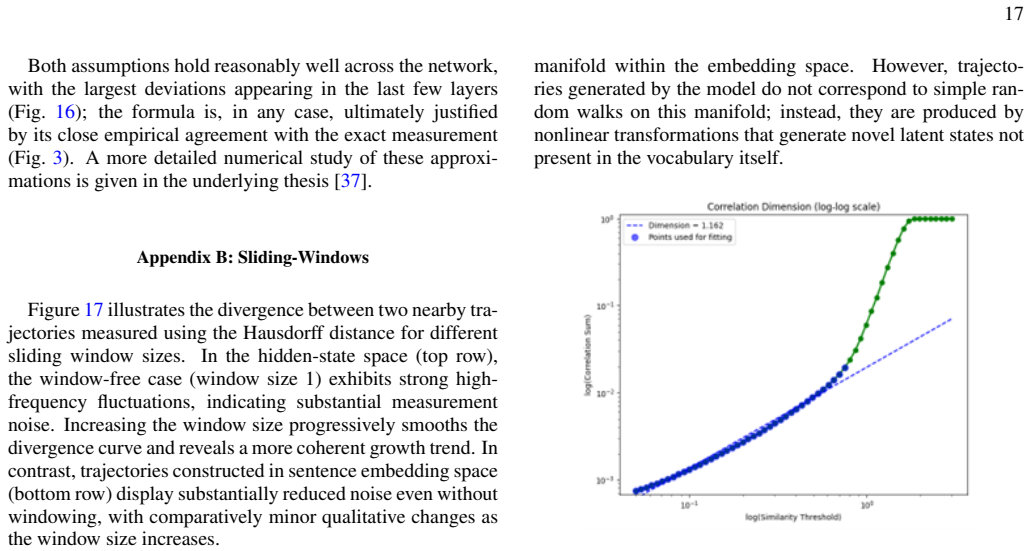
- [V.E, Eq. (21)] The Grassberger–Procaccia correlation dimension is applied to raw, serially correlated trajectory points without Theiler-type temporal decorrelation, explicit scaling-region selection, or surrogate analysis. For short, high-dimensional, autocorrelated trajectories, the slope of C(ε) can mimic a low fractal dimension even for stochastic or quasi-periodic signals. The random-vector comparison in Fig. 14 is not a surrogate control because it destroys temporal correlations. Report D2 with a Theiler window, bootstrap confidence intervals, and surrogate comparisons; otherwise the fractal-attractor conclusion is unsupported.
- [V.A.1.a, Eq. (30)] The text and conclusion describe Eq. (30) as a 'predictive, weight-only' formula, but it depends on measured activation densities s_x,d_x from the same forward pass used for validation (Fig. 3). As a closed-form reorganization of the Jacobian it is useful, but as a predictor it is circular. Test it on held-out inputs or reframe it as a diagnostic decomposition; also state explicitly which quantities are static weights and which are data-dependent.
- [Appendix D / V.A.5] The perturbation magnitude r∈[2.5×10^-4, 5×10^-4] overlaps or lies below the reported FP16 activation spacing (≈4.88×10^-4 in [0.5,1.0]-scale activations). The paper does not show that the injected embedding-space perturbation remains above the rounding noise of the actual pipeline. Please quantify the effective perturbation after FP16 quantization, compare with a perturbation-free control (e.g., two runs with identical inputs under FP32/FP64), and verify the divergence phenomenology in higher precision. This is necessary to rule out numerical noise as the source of the 'nearby' trajectory differences.
minor comments (6)
- [Fig. 7 caption] The caption uses 'Lyapunov timeseries' and 'lyapunov exponent' for what is actually a finite-time local slope of log-distance. Please use 'finite-time exponent' or 'local divergence rate' to avoid conflating this with the true Lyapunov exponent.
- [Eq. (33)] The equation uses a continuous derivative d/dt but the data are discrete. Specify the finite-difference estimator used to compute the slope.
- [V.C, Fig. 11] The non-monotonic attention-window curve is a key causal claim, but the figure appears to show a single ensemble/prompt. Add error bars, number of prompts, and statistical significance, and state the perturbation magnitude used (the text says 10^-4, while Appendix D lists 3.5–4×10^-4).
- [Abstract and Conclusions] The phrase 'hallmark signatures of chaos' is stronger than what Sec. V.B delivers. Consider phrasing such as 'chaos-like signatures' or 'sensitivity consistent with chaos' unless a Lyapunov-based discriminator is added.
- [Data Availability] The statement 'available from the corresponding author upon reasonable request' limits reproducibility. I recommend releasing code, trajectories, and recurrence plots, especially since several thresholds and scaling regions are chosen manually.
- [References] Reference [48] appears as a numbered footnote-like entry rather than a proper reference; several preprints are undated or have future arXiv numbers (e.g., [15], [17], [18]) — please add accessible identifiers and dates in the final version.
Circularity Check
Central chaos claim is interpretive, not circular; one secondary step — the mean-field λ̄ formula (Eq. 30) — is validated against its own inputs and mislabeled a 'predictive, weight-only diagnostic'.
specific steps
-
self definitional
[Sec. V.A.1.a (Eq. 30, Fig. 3) and Sec. VI (Conclusions)]
"yields a closed-form estimate for the isotropic expansion that requires only the static weight norms and the activation densities (full derivation in Appendix A): λ̄≈ F̃_down[F̃_gate d²_x + F̃_up s²_x]. (30) Fig. 3 shows that this simple closed-form estimate tracks the exact, empirically measured expansion factor across all layers... giving a predictive, weight-only diagnostic for a component’s contribution to chaotic stretching."
The 'predicted' expansion factor is not weight-only and is not an out-of-sample prediction. Eq. 30's inputs — activation densities s²_x, d²_x — are measured from the same forward pass whose exact Jacobian expansion λ̄ = ||J(x)||²_F/D is the validation target in Fig. 3. Since the exact λ̄ is itself a function of those same activations, the formula is an algebraic/mean-field approximation of the measured quantity from its own inputs; the agreement checks the mean-field assumptions (Fig. 16) rather than predicting a new quantity. The Sec. VI 'predictive, weight-only' claim overstates an approximation identity.
full rationale
The central claim — that LLM inference exhibits chaotic signatures (sensitivity, boundedness, recurrence, fractal dimensionality) — is an interpretation of independent measurements, not a tautology. The paper defines chaos in Sec. III.A via exponential divergence (Eq. 3, λ>0) and then concedes the defining test is unavailable: 'the discreteness of the token space prevents a robust global estimate of the maximal Lyapunov exponent' and 'we do not observe a smooth increase of the distance but instead it is always characterized by large jumps' (Sec. V.B). That the latent-then-jump pattern, with a negative pre-flip finite-time exponent and post-flip divergence driven by differing context tokens, may under-support the chaos classification is a validity concern, not circularity: the paper does not define chaos as jumpiness but appeals to an analogy with discrete-space chaotic systems. The operator-level Jacobian analysis (Sec. V.A, Eqs. 28–32) is exact mathematics on the model's own architecture plus a matrix-free numerical estimate, and the attention-window experiment (Sec. V.C) is a genuine control manipulation; neither reduces to its own conclusions. Self-citations ([37], the first author's BSc thesis) appear only for replication details and numerical study of approximations — not load-bearing for the central derivation. The one concrete circular step is the mean-field feed-forward formula (Eq. 30): its inputs (activation densities) come from the same forward pass against which it is validated (Fig. 3), making the agreement an approximation identity rather than an independent prediction, and the 'weight-only' characterization is inaccurate. Because this affects a secondary supporting diagnostic rather than the central claim, the overall circularity is mild.
Axiom & Free-Parameter Ledger
free parameters (4)
- Initial perturbation magnitude r =
3.5×10⁻⁴ / 4×10⁻⁴ (App. D)
- Recurrence rate threshold =
0.03 (Fig. 12), 0.05 (Fig. 13)
- Lyapunov fit interval and sliding window w =
pre-saturation interval; w=16 (claimed robust for w∈{8,32})
- GP correlation-dimension scaling region =
unspecified linear region in log–log plot
axioms (5)
- domain assumption Autoregressive inference under greedy decoding (T=0) defines a deterministic discrete-time map F on hidden states.
- domain assumption Grassberger–Procaccia on raw trajectory points (no delay embedding, no Theiler window) yields valid correlation dimensions for these autocorrelated, non-stationary text-generated sequences.
- ad hoc to paper Visual similarity of recurrence plots to the Lorenz attractor is diagnostic of deterministic chaos.
- domain assumption Mean-field simplifications of Appendix A: off-diagonal Gramian terms destructively interfere; weight norms are approximately uniform.
- ad hoc to paper The injected perturbation of norm r≈3.5–4×10⁻⁴ survives the numerical precision of the pipeline and is amplified deterministically rather than drowned in FP16 rounding.
read the original abstract
Large Language Models (LLMs) have achieved remarkable performance across a wide range of tasks, yet their internal dynamics remain poorly understood. In this work, we apply the tools of nonlinear dynamics and chaos theory to LLMs. By analyzing both text and hidden state trajectories, we demonstrate that LLMs exhibit hallmark signatures of chaos, including strong sensitivity to initial conditions, manifested as intermittent, jump-like divergence of nearby trajectories combined with bounded evolution, with consistent results across different distance metrics. An exact Jacobian analysis of the Transformer's sub-blocks shows that self-attention and the feed-forward network expand and propagate perturbations, while normalization and residual connections counteract this expansion and promote stability. Recurrence plots show structural similarities between LLMs and canonical chaotic systems such as the Lorenz attractor, while dimension analysis reveals fractal structures in the hidden state space, particularly pronounced in the last layers. We propose that the nonlinear coupling induced by attention mechanisms plays a key role in driving this chaotic behavior.
Figures



Reference graph
Works this paper leans on
-
[1]
Vaswani, N
A. Vaswani, N. Shazeer, N. Parmar, J. Uszkoreit, L. Jones, A. N. Gomez, L. u. Kaiser, and I. Polosukhin, inAdvances in Neural Information Processing Systems, V ol. 30, edited by I. Guyon, U. V . Luxburg, S. Bengio, H. Wallach, R. Fergus, S. Vish- wanathan, and R. Garnett (Curran Associates, Inc., 2017)
2017
-
[2]
Chain-of-thought prompting elicits reasoning in large language models,
J. Wei, X. Wang, D. Schuurmans, M. Bosma, B. Ichter, F. Xia, E. Chi, Q. Le, and D. Zhou, “Chain-of-thought prompting elicits reasoning in large language models,” (2023), arXiv:2201.11903 [cs.CL]
Pith/arXiv arXiv 2023
-
[3]
X. Li, Y . Leng, R. Ding, H. Mo, and S. Yang, arXiv preprint arXiv:2503.13530 (2025)
Pith/arXiv arXiv 2025
-
[4]
A mathematical perspective on transformers,
B. Geshkovski, C. Letrouit, Y . Polyanskiy, and P. Rigol- let, “A mathematical perspective on transformers,” (2025), arXiv:2312.10794 [cs.LG]
Pith/arXiv arXiv 2025
-
[5]
Dynamical mean- field theory of self-attention neural networks,
Ángel Poc-López and M. Aguilera, “Dynamical mean- field theory of self-attention neural networks,” (2024), arXiv:2406.07247 [cond-mat.dis-nn]
Pith/arXiv arXiv 2024
- [6]
-
[7]
Sompolinsky, A
H. Sompolinsky, A. Crisanti, and H. J. Sommers, Physical Re- view Letters61, 259 (1988)
1988
-
[8]
Bertschinger and T
N. Bertschinger and T. Natschläger, Neural Computation16, 1413 (2004)
2004
-
[9]
Exponential expressivity in deep neural networks through transient chaos,
B. Poole, S. Lahiri, M. Raghu, J. Sohl-Dickstein, and S. Gan- guli, “Exponential expressivity in deep neural networks through transient chaos,” (2016), arXiv:1606.05340 [stat.ML]
Pith/arXiv arXiv 2016
-
[10]
S. S. Schoenholz, J. Gilmer, S. Ganguli, and J. Sohl-Dickstein, “Deep information propagation,” (2017), arXiv:1611.01232 [stat.ML]
Pith/arXiv arXiv 2017
-
[11]
Mean field residual networks: On the edge of chaos,
G. Yang and S. S. Schoenholz, “Mean field residual networks: On the edge of chaos,” (2017), arXiv:1712.08969 [stat.ML]
Pith/arXiv arXiv 2017
-
[12]
M. Chen, J. Pennington, and S. S. Schoenholz, “Dynam- ical isometry and a mean field theory of rnns: Gating en- ables signal propagation in recurrent neural networks,” (2018), arXiv:1806.05394 [stat.ML]
Pith/arXiv arXiv 2018
-
[13]
The lipschitz con- stant of self-attention,
H. Kim, G. Papamakarios, and A. Mnih, “The lipschitz con- stant of self-attention,” (2021), arXiv:2006.04710 [stat.ML]
Pith/arXiv arXiv 2021
-
[14]
Softmax is 1/2-lipschitz: A tight bound across allℓ p norms,
P. Nair, “Softmax is 1/2-lipschitz: A tight bound across allℓ p norms,” (2025), arXiv:2510.23012 [cs.LG]
arXiv 2025
-
[15]
Exact attention sensitivity and the geometry of transformer stability,
S. M. Emadi, “Exact attention sensitivity and the geometry of transformer stability,” (2026), arXiv:2602.18849 [cs.LG]
arXiv 2026
-
[16]
Stabilizing trans- former training by preventing attention entropy collapse,
S. Zhai, T. Likhomanenko, E. Littwin, D. Busbridge, J. Rama- puram, Y . Zhang, J. Gu, and J. Susskind, “Stabilizing trans- former training by preventing attention entropy collapse,” (2023), arXiv:2303.06296 [cs.LG]
Pith/arXiv arXiv 2023
-
[17]
Spectral conditioning of attention improves transformer performance,
H. Saratchandran and S. Lucey, “Spectral conditioning of attention improves transformer performance,” (2026), arXiv:2603.07162 [cs.LG]
arXiv 2026
-
[18]
Dynamics of the transformer residual stream: Coupling spectral geometry to network topol- ogy,
J. Fernando and G. Guitchounts, “Dynamics of the transformer residual stream: Coupling spectral geometry to network topol- ogy,” (2026), arXiv:2605.14258 [cs.LG]
Pith/arXiv arXiv 2026
-
[19]
H. He and T. M. Lab, Thinking Machines Lab: Connectionism (2025), 10.64434/tml.20250910, https://thinkingmachines.ai/blog/defeating-nondeterminism-in- llm-inference/
-
[20]
Z. Wang, Y . Li, J. Yan, Y . Cheng, and Y . Zhang, arXiv preprint arXiv:2502.15208 (2025)
Pith/arXiv arXiv 2025
-
[21]
Tanaka and Y
T. Tanaka and Y . Yamaguti, PLOS Complex Systems2, 1 (2025)
2025
-
[22]
Sussillo and O
D. Sussillo and O. Barak, Neural Computation25, 626 (2013)
2013
-
[23]
S. Zhang, A. Patel, S. A. Rizvi, N. Liu, S. He, A. Karbasi, E. Zappala, and D. van Dijk, arXiv preprint arXiv:2410.02536 (2024)
Pith/arXiv arXiv 2024
-
[24]
The geometry of reasoning: Flowing logics in representation space,
Y . Zhou, Y . Wang, X. Yin, S. Zhou, and A. R. Zhang, “The geometry of reasoning: Flowing logics in representation space,” (2025), arXiv:2510.09782 [cs.AI]
arXiv 2025
-
[25]
C. Olah, N. Cammarata, L. Schubert, G. Goh, M. Petrov, and S. Carter, Distill (2020), 10.23915/distill.00024.001, https://distill.pub/2020/circuits/zoom-in
-
[26]
Ameisen, J
E. Ameisen, J. Lindsey, A. Pearce, W. Gurnee, N. L. Turner, B. Chen, C. Citro, D. Abrahams, S. Carter, B. Hosmer, J. Mar- cus, M. Sklar, A. Templeton, T. Bricken, C. McDougall, H. Cunningham, T. Henighan, A. Jermyn, A. Jones, A. Persic, Z. Qi, T. Ben Thompson, S. Zimmerman, K. Rivoire, T. Con- erly, C. Olah, and J. Batson, Transformer Circuits Thread (2025)
2025
-
[27]
Lindsey, W
J. Lindsey, W. Gurnee, E. Ameisen, B. Chen, A. Pearce, N. L. Turner, C. Citro, D. Abrahams, S. Carter, B. Hosmer, J. Marcus, M. Sklar, A. Templeton, T. Bricken, C. McDougall, H. Cunningham, T. Henighan, A. Jermyn, A. Jones, A. Persic, Z. Qi, T. B. Thompson, S. Zimmerman, K. Rivoire, T. Conerly, C. Olah, and J. Batson, Transformer Circuits Thread (2025)
2025
-
[28]
Selivanov, M
D. Selivanov, M. Bickel, and Q. Wang,text2vec: Modern Text Mining Framework for R(2024), r package version 0.6.4
2024
-
[29]
Sentence-bert: Sentence embed- dings using siamese bert-networks,
N. Reimers and I. Gurevych, “Sentence-bert: Sentence embed- dings using siamese bert-networks,” (2019), arXiv:1908.10084 [cs.CL]
Pith/arXiv arXiv 2019
-
[30]
Salvador and P
S. Salvador and P. Chan, Intelligent Data Analysis11, 561 (2007)
2007
-
[31]
frechetdist: A Python implementation of the discrete Fréchet distance algorithm,
S. Denaxas, “frechetdist: A Python implementation of the discrete Fréchet distance algorithm,”https://pypi.org/ project/frechetdist/(2023), accessed: 2025-10-20
2023
-
[32]
Eiter and H
T. Eiter and H. Mannila,Computing discrete Fréchet distance, Tech. Report CD-TR 94/64 (Information Systems Department, 16 Technical University of Vienna, 1994)
1994
-
[33]
scipy.spatial.distance.directed_hausdorff — scipy v1.16.2 manual,
T. S. Community, “scipy.spatial.distance.directed_hausdorff — scipy v1.16.2 manual,”https://docs.scipy.org/ doc/scipy/reference/generated/scipy.spatial. distance.directed_hausdorff.html(2024), accessed: 2025-10-20
2024
-
[34]
Grassberger and I
P. Grassberger and I. Procaccia, Physica D: Nonlinear Phenom- ena9, 189 (1983)
1983
-
[35]
Deepseek-r1-distill-qwen-1.5b,
DeepSeek-AI, “Deepseek-r1-distill-qwen-1.5b,” https://huggingface.co/deepseek-ai/ DeepSeek-R1-Distill-Qwen-1.5B(2025), distilled model based on Qwen architecture and DeepSeek-R1 teacher
2025
-
[36]
Phi-4-mini technical re- port: Compact yet powerful multimodal language models via mixture-of-loras,
Microsoft, A. Abouelenin,et al., “Phi-4-mini technical re- port: Compact yet powerful multimodal language models via mixture-of-loras,” (2025), arXiv:2503.01743 [cs.CL]
Pith/arXiv arXiv 2025
-
[37]
Jaca,Chaos in Large Language Models, BSc thesis, Bu- dapest University of Technology and Economics (2026)
G. Jaca,Chaos in Large Language Models, BSc thesis, Bu- dapest University of Technology and Economics (2026)
2026
-
[38]
We compared the results using three different embedding models:all-mpnet-base-v2,intfloat/e5-large-v2, and facebook/contriever, with no significant differences be- tween them
-
[39]
This also explains why cosine-based metrics, insensitive to the (normalized-away) radial direction, are particularly well suited to LLM hidden states, cf. Sec. IV A
-
[40]
K. Ethayarajh, inProceedings of the 2019 conference on em- pirical methods in natural language processing and the 9th international joint conference on natural language processing (EMNLP-IJCNLP)(2019) pp. 55–65
2019
-
[41]
W. Rudman and C. Eickhoff, arXiv preprint arXiv:2305.19358 (2023)
Pith/arXiv arXiv 2023
-
[42]
E. N. Lorenz, Journal of Atmospheric Sciences20, 130 (1963)
1963
-
[43]
Distributions of angles in random packing on spheres,
T. Cai, J. Fan, and T. Jiang, “Distributions of angles in random packing on spheres,” (2013), arXiv:1306.0256 [math.ST]
Pith/arXiv arXiv 2013
-
[44]
A. N. Gorban and I. Y . Tyukin, Philosophical Transactions of the Royal Society A: Mathematical, Physical and Engineering Sciences376, 20170237 (2018)
2018
-
[45]
The linear representa- tion hypothesis and the geometry of large language models,
K. Park, Y . J. Choe, and V . Veitch, “The linear representa- tion hypothesis and the geometry of large language models,” (2024), arXiv:2311.03658 [cs.CL]
Pith/arXiv arXiv 2024
-
[46]
Boedecker, O
J. Boedecker, O. Obst, J. Lizier, N. Mayer, and M. Asada, The- ory in Biosciences131, 205 (2012)
2012
-
[47]
C. G. Langton, Physica D: Nonlinear Phenomena42, 12 (1990)
1990
-
[48]
It is trained and fine-tuned to replicate the behavior from the DeepSeek R1
The model used is distilled from DeepSeek R1 reducing the number of parameters from 671 billion to 1.5 billion. It is trained and fine-tuned to replicate the behavior from the DeepSeek R1. This distilled model is based on the Qwen2.5 family and there are differences in the architecture, which are beyond the scope of this study. All the points mentioned in...
-
[49]
From below, the perturbation must ex- ceed the FP16 numerical noise floor of the inference pipeline (≈5×10 −4 in activation space, cf
[48] •Temperature:0 (to ensure determinism) •Sampling:greedy (to ensure determinism) •Context Window:3096 tokens •Initial Perturbation Magnitude:0.00035 or 0.0004 •Vocabulary Size:151936 •Hidden/Embedding Dimension:1536 •Attention Heads:12 •Hidden Layers:28 The choice of the initial perturbation magnituderis not arbitrary: its admissible range is bounded ...
2000
discussion (0)
Sign in with ORCID, Apple, or X to comment. Anyone can read and Pith papers without signing in.