REVIEW 3 major objections 4 minor 47 references
A continuous-time quantum walk on feasible vertex covers can rank vertices well enough to guide greedy reductions that beat degree-based classical greedy on tested random graphs.
Reviewed by Pith at T0; open to challenge. T0 means a machine referee read the full paper against a public rubric. the ladder, T0–T4 →
T0 review · deepseek-v4-flash
2026-07-31 23:05 UTC pith:JS5OCNYU
load-bearing objection Clean construction, honest benchmarks, one calibration-robustness soft spot that should not block peer review. the 3 major comments →
Iterative quantum algorithms for the minimum vertex cover problem based on continuous-time quantum walks
The pith
A machine-rendered reading of the paper's core claim, the machinery that carries it, and where it could break.
Core claim
Restricted to the feasible subspace, the projected Pauli-X Hamiltonian H_MVC = Σ_i Π_{N(i)} X_i coincides with the adjacency matrix of the induced feasible-state graph G_VC(G), whose vertices are feasible covers and whose edges are feasibility-preserving single-bit flips. Since every feasible cover is reachable from the all-in cover, a continuous-time quantum walk starting there explores all covers without ever leaving feasibility. The paper shows numerically that direct sampling of a minimum cover is exponentially suppressed in system size, but the walk's per-vertex marginals and conditioned energies encode global structural information through a light-cone of nested commutators. Using thos
What carries the argument
The central object is H_MVC = Σ_i Π_{N(i)} X_i, where the projector Π_{N(i)} requires all neighbours of i to already be in the cover, so flipping i can never uncover an edge. Restricted to the feasible subspace, H_MVC equals the adjacency matrix of the induced feasible-state graph G_VC(G). This identification turns the unitary e^{itH_MVC} into a continuous-time quantum walk on the layered graph of feasible covers, and the walk state provides vertex scores — marginal probabilities P_v or conditioned expected costs E_v — that drive a recursive greedy reduction. The connectivity theorem ensures every feasible cover is reachable from the all-in cover by allowed flips.
Load-bearing premise
The benchmark conclusions depend on a single walk duration calibrated on 100 small graphs per family and then reused at every graph size, every circuit depth, and every recursive step, even though the residual graph shrinks as vertices are fixed.
What would settle it
Take held-out 3-regular graphs at n=20. Run QEG-LDF with the n=18-calibrated walk time; run it again with t chosen by grid search on n=20; and run a classical degree-based greedy that is allowed the same kind of per-family tuning. If the fixed-time quantum variant is not better than the tuned classical baseline, the reported advantage is an artifact of calibration transfer.
If this is right
- MIS is handled with the same machinery: bitwise complementation turns vertex covers into independent sets, so the constraint-preserving walk and greedy reduction transfer without new penalty terms.
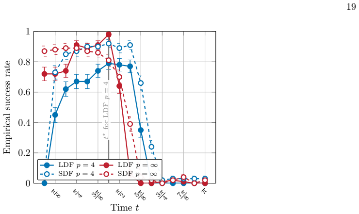
- For bounded-degree graphs, each Trotter layer of the walk has circuit depth independent of system size, and depth p=4 already tracks the exact evolution closely for QEG; shallow circuits suffice on the tested families.
- The limiting resource is measurement: QEG requires one conditioned circuit per candidate vertex per recursive step, so the practical trade-off is score stability versus circuit-evaluation count.
- Direct single-shot extraction of an optimal cover from the walk is not the right operating point; the useful quantum output is a ranking of vertices, not a solution state.
- The p=1 Monte Carlo surrogate extends the same scores to graphs of hundreds of vertices, so the framework can be probed beyond exact-state sizes.
Where Pith is reading between the lines
- An extension the authors leave implicit is adaptive walk-time selection: because the walk time is fixed from a calibration ensemble and not rescaled as the residual graph shrinks, recalibrating t at each recursion level is a natural next test and may change the size of the reported advantage.
- At p=1 the quantum circuit reduces to a classical sequential removal process with removal probability determined by cos²(t); a classical probabilistic greedy with the same per-vertex tie-breaking would isolate how much of the gain comes from coherent multi-qubit interference rather than from the sequential pruning rule.
- The layered-transport analysis suggests that cumulative probability in the bottom few layers saturates quickly, implying that per-vertex rankings stay informative at sizes where full quantum simulation is impossible; this could be tested by running the Monte Carlo surrogate at n beyond 300 and watching whether the gap to classical baselines widens or narrows.
- The O(V^2) conditioned-circuit count of QEG motivates adaptive shot allocation, since scores are evaluated as exact expectation values in the paper; finite-shot estimation of small score gaps is likely the dominant hardware cost.
Editorial analysis
A structured set of objections, weighed in public.
Referee Report
Summary. The paper proposes a penalty-free hybrid quantum-classical greedy framework for minimum vertex cover. The key construction is a projected-Pauli-X Hamiltonian whose restriction to the feasible subspace is the adjacency matrix of the induced graph of feasible covers; the authors prove that this graph is connected from the all-in cover and that a continuous-time quantum walk on it can be used to define vertex scores. Two score families are developed: QPG (marginal occupation probabilities) and QEG (conditioned expected cover size), each combined with LDF-like and SDF-like recursive reduction rules. Numerical benchmarks on 3-regular, 4-regular, and Erdős–Rényi graphs (n=8..20) compare the LDF variants against classical greedy baselines and FastVC, with walk times calibrated on independent n=18 ensembles. The paper also contains Trotter-depth analysis, a p=1 Monte Carlo surrogate up to n=300, and a Lean 4 formalization of support bookkeeping.
Significance. If the empirical claims hold, the paper gives a clean and conceptually appealing way to convert constrained continuous-time quantum walks into local greedy signals, without penalty terms or variational training. The structural results—Theorem 1, Corollary 1, Eq. (3), Proposition 1, and the parity selection rule—are mathematically sound and are partly machine-checked. The paper is honest about its calibration protocol, releases code and data, and explicitly separates the mathematical core from the heuristic benchmark contribution. However, the central empirical advantage is asserted for the LDF variants only, and the fixed calibrated walk time is transferred across sizes, Trotter depths, and recursion levels without a robustness analysis; this makes the headline claim less secure than the abstract suggests.
major comments (3)
- [Section VI.C, Eq. (10), Figures 7 and 9] The benchmark conclusion relies on a single calibrated walk time t* per (family, score, rule), selected on 100 n=18 instances and then used for every n in {8,...,20}, every finite Trotter depth, and every recursion level. This is a non-trivial transfer because the induced-graph depth D(G)=n-τ(G) changes with system size and shrinks during recursion, and Figures 4 and 7 indicate that the optimal contrast time depends on the layer structure. The paper discloses this and lists adaptive walk-time selection as future work, but it does not test whether the reported advantage is robust to the fixed choice. Please add a sensitivity analysis—for example, success-rate-vs-t curves for several sizes, per-size calibration, or rescaling t by D(G)—or explicitly restrict the claim to the tested fixed-time protocol. Without such an analysis, the empirical conclusion is contingent on an unexamined hyperpa
- [Section VI.B, Figure 11, abstract] The abstract claims that 'the quantum-informed algorithms achieve lower mean approximation ratios and solve a larger fraction of instances optimally than their corresponding classical greedy baselines.' Figure 11, however, compares only QPG-LDF and QEG-LDF against Greedy LDF, Greedy SDF, and FastVC; the SDF-like variants (QPG-SDF and QEG-SDF) are not shown against Greedy SDF in that figure. Figures 7, 9, and 10 present the SDF variants only among themselves. Thus the plural claim is not directly supported for the SDF rules. Either add the SDF-vs-Greedy-SDF comparison or qualify the abstract and conclusion to state that the demonstrated advantage is for the LDF variants.
- [Section VI.B, Fig. 11 caption] The figure caption states 'for n=18' while the horizontal axis runs over n=8,10,...,20. This is not merely a typo: it obscures whether the panel is aggregated over all sizes or only at n=18. If the panels are aggregated over sizes, the caption should say so; if they are per-size, the x-axis is redundant. Please clarify.
minor comments (4)
- [Section V.A vs Section VI.A] Section V.A says that for QPG the gap between p=4 and p=∞ is substantial, while Section VI.A says that already at p=4 the LDF performance is close to the exact evolution. The apparent tension should be reconciled, e.g., by distinguishing score fidelity from final success rate.
- [Eq. (10)] The notation bPopt is used before its full definition is given. Please introduce it explicitly as the empirical success rate on the calibration ensemble.
- [Section VI, first paragraph] The sentence about measurement shots appears parenthetically. Since the benchmarks use exact expectation values, it would be clearer to state explicitly in the results section that shot noise is not included in any figure, and to mention the resulting uncertainty in the conclusion.
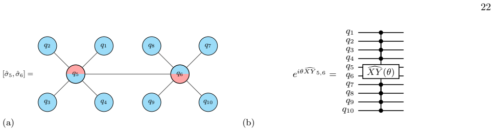
- [Appendix D, Fig. 18] The p=1 Monte Carlo results are a useful extension, but the caption and text should more strongly emphasize that these are classical simulations of a quantum-inspired rule and do not constitute evidence of a quantum speedup. The current wording already says this, but the placement in a figure-heavy appendix may allow readers to over-interpret.
Circularity Check
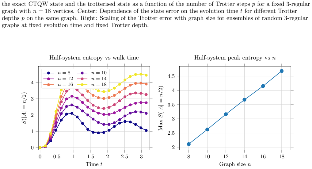
No significant circularity: the central derivation is self-contained; the only calibrated quantity (walk time t*) is selected on disjoint calibration ensembles and then applied to held-out benchmarks.
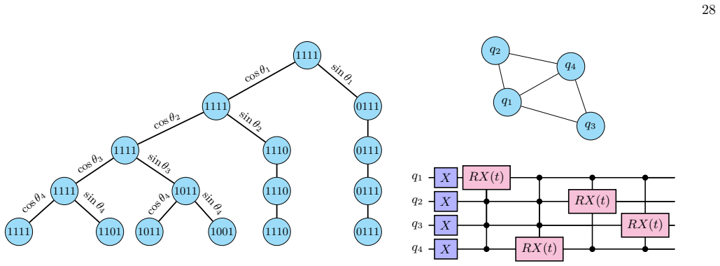
full rationale
The paper's mathematical core — the reachability theorem, the induced feasible-state graph, and the identification of the projected-Pauli Hamiltonian with the adjacency matrix of that graph — is derived from the definitions of the vertex-cover feasibility projector and the neighbourhood-controlled operators, not from the target result. Equation (3), H_MVC restricted to H_VC equals A(G_VC(G)), is an exact algebraic reformulation by construction, not a fitted or predicted output. The QPG and QEG scores are explicit expectation values: P_v(t) is the marginal occupation of the CTQW state and E_v(t) is the conditioned expected cost; neither is defined in terms of the benchmark outcome or the optimal cover. The only fitted quantity is the walk time t*, selected in Eq. (10) by maximizing the empirical success rate on independent calibration ensembles of 100 n=18 instances. The paper explicitly states that these calibration ensembles are disjoint from every benchmark ensemble used in figure 11, and that all benchmark points are evaluated on held-out ensembles. Using a hyperparameter tuned on a separate calibration set to evaluate held-out instances is standard hyperparameter calibration, not circular reasoning: the benchmark success rates are not equal by construction to the calibration objective. The paper also discloses the limitation that t* is not rescaled as the residual graph shrinks and lists adaptive walk-time selection as an open question; this is a robustness/transfer concern about the empirical comparison, not a circularity. Self-citations such as [12] and [17] are not load-bearing for the central claim: the projected Pauli mixers are attributed to the external reference [14], and the connectivity result is proved in the paper itself, with the support bookkeeping additionally machine-verified in Lean 4. No step in the paper's derivation chain reduces to its own input, and no fitted parameter is renamed as a prediction. The reported quantum advantage is an empirical benchmark result conditional on calibrated hyperparameters, not a conclusion forced by definition or by a self-citation chain.
Axiom & Free-Parameter Ledger
free parameters (2)
- Walk time t*_{s,R,f} =
not stated numerically; chosen from grid {0, π/16, ..., π} via Eq. (10)
- Trotter depth p=4 for headline benchmarks =
4
axioms (6)
- standard math The projected Pauli-X operators \hat X_i = Π_{N(i)} X_i preserve the feasible vertex-cover subspace, and the restricted Hamiltonian H_MVC equals the adjacency matrix of the induced feasible-state graph.
- standard math The reference state |Ω> = |1>^⊗n is a feasible cover, and every feasible cover is reachable from it by constraint-preserving single flips.
- standard math First-order Suzuki–Trotter error is O(|E|t^2/p) and supports the low-depth approximations used in benchmarks.
- domain assumption For bounded-degree graphs, each Trotter layer can be implemented in constant depth using ancilla-free multi-controlled SU(2) decompositions.
- domain assumption Calibration ensembles are independent of benchmark ensembles and representative of the three graph families.
- ad hoc to paper The walk-time grid {0, π/16, ..., π} contains a good operating point for each family.
read the original abstract
We introduce a constraint-preserving hybrid quantum-classical greedy framework for the minimum vertex cover problem, which extends directly to maximum independent set by bitwise complementation. The framework uses projected Pauli-X terms whose sum preserves the feasible subspace and acts within it exactly as the adjacency matrix of a layered graph of feasible covers. This graph is connected, so every feasible cover is linked to the configuration containing all vertices by a sequence of allowed single-vertex flips. Starting from this configuration, the corresponding continuous-time quantum walk propagates amplitude into layers containing progressively smaller covers. We rank vertices using either their marginal cover probabilities or the expected cover size obtained after fixing each candidate vertex in the cover, and use these rankings to guide recursive greedy reductions. Across several random-graph families, with walk times fixed using independent calibration ensembles, the quantum-informed algorithms achieve lower mean approximation ratios and solve a larger fraction of instances optimally than their corresponding classical greedy baselines. The conditioned-energy strategy performs best on the tested instances and retains algorithmic performance close to the exact continuous-time limit under low-depth Trotterisation. For bounded-degree graphs, each Trotter layer has circuit depth independent of system size, and the framework requires neither penalty terms nor variational training.
Figures



Reference graph
Works this paper leans on
-
[1]
R. M. Karp, Reducibility among combinatorial problems, in50 Years of Integer Programming 1958-2008: from the Early Years to the State-of-the-Art(Springer, 2009) pp. 219–241
1958
-
[2]
V. V. Vazirani,Approximation algorithms, Vol. 1 (Springer, 2001)
2001
-
[3]
Khot, On the power of unique 2-prover 1-round games, inProceedings of the thiry-fourth annual ACM sympo- sium on Theory of computing(2002) pp
S. Khot, On the power of unique 2-prover 1-round games, inProceedings of the thiry-fourth annual ACM sympo- sium on Theory of computing(2002) pp. 767–775
2002
-
[4]
Halld´ orsson and J
M. Halld´ orsson and J. Radhakrishnan, Greed is good: Approximating independent sets in sparse and bounded- degree graphs, Algorithmica (New York)18, 145 (1997)
1997
-
[5]
Krysta, M
P. Krysta, M. Mari, and N. Zhi, Ultimate greedy approxi- mation of independent sets in subcubic graphs, Algorith- mica86, 3518 (2024)
2024
-
[6]
T. A. Feo and M. G. C. Resende, Greedy randomized adaptive search procedures, Journal of Global Optimiza- tion6, 109 (1995)
1995
-
[7]
Bang-Jensen, G
J. Bang-Jensen, G. Gutin, and A. Yeo, When the greedy algorithm fails, Discrete Optimization1, 121 (2004)
2004
-
[8]
Lucas, Ising formulations of many np problems, Fron- tiers in Physics2, 5 (2014)
A. Lucas, Ising formulations of many np problems, Fron- tiers in Physics2, 5 (2014)
2014
-
[9]
E. Pelofske, G. Hahn, and H. Djidjev, Solving large min- imum vertex cover problems on a quantum annealer, arXiv:1904.00051 (2019)
Pith/arXiv arXiv 1904
-
[10]
E. Farhi, J. Goldstone, and S. Gutmann, A quan- tum approximate optimization algorithm, arXiv (2014), arXiv:1411.4028 [quant-ph]
Pith/arXiv arXiv 2014
-
[11]
Peruzzo, J
A. Peruzzo, J. McClean, P. Shadbolt, M.-H. Yung, X.-Q. Zhou, P. J. Love, A. Aspuru-Guzik, and J. L. O’brien, A variational eigenvalue solver on a photonic quantum processor, Nature communications5, 4213 (2014)
2014
-
[12]
F. G. Fuchs, K. O. Lye, H. Møll Nilsen, A. J. Stasik, and G. Sartor, Constraint preserving mixers for the quantum approximate optimization algorithm, Algorithms15, 202 (2022)
2022
-
[13]
Herman, R
D. Herman, R. Shaydulin, Y. Sun, S. Chakrabarti, S. Hu, P. Minssen, A. Rattew, R. Yalovetzky, and M. Pistoia, Constrained optimization via quantum zeno dynamics, Communications Physics6, 219 (2023)
2023
-
[14]
S. Hadfield, Z. Wang, B. O’Gorman, E. G. Rieffel, D. Venturelli, and R. Biswas, From the quantum ap- proximate optimization algorithm to a quantum alternat- ing operator ansatz, Algorithms12, 10.3390/a12020034 (2019)
-
[15]
Z. Wang, N. C. Rubin, J. M. Dominy, and E. G. Rief- fel, XY mixers: Analytical and numerical results for the quantum alternating operator ansatz, Phys. Rev. A101, 012320 (2020). 17
2020
-
[16]
A. B¨ artschi and S. Eidenbenz, Grover mixers for qaoa: Shifting complexity from mixer design to state prepara- tion, arXiv:2006.00354 (2020)
Pith/arXiv arXiv 2006
-
[17]
F. G. Fuchs and R. P. Bassa, Lx-mixers for qaoa: Op- timal mixers restricted to subspaces and the stabilizer formalism, Quantum8, 1535 (2024)
2024
-
[18]
Z. H. Saleem, Max-independent set and the quantum al- ternating operator ansatz, International Journal of Quan- tum Information18, 2050011 (2020)
2020
-
[19]
Bucher, J
D. Bucher, J. Stein, S. Feld, and C. Linnhoff-Popien, Penalty-free approach to accelerating constrained quan- tum optimization, Physical Review A112, 062605 (2025)
2025
-
[20]
Montanaro, Quantum speedup of branch-and-bound algorithms, Physical Review Research2, 013056 (2020)
A. Montanaro, Quantum speedup of branch-and-bound algorithms, Physical Review Research2, 013056 (2020)
2020
-
[21]
S. Chakrabarti, P. Minssen, R. Yalovetzky, and M. Pistoia, Universal quantum speedup for branch- and-bound, branch-and-cut, and tree-search algorithms, arXiv preprint arXiv:2210.03210 (2022)
Pith/arXiv arXiv 2022
-
[22]
S. Wilkening, A.-I. Lefterovici, L. Binkowski, M. Perk, S. P. Fekete, and T. J. Osborne, A quantum algorithm for solving 0-1 knapsack problems, npj Quantum Infor- mation11, 10.1038/s41534-025-01097-8 (2025)
-
[23]
D. J. Egger, J. Mareˇ cek, and S. Woerner, Warm-starting quantum optimization, Quantum5, 479 (2021)
2021
-
[24]
Bravyi, A
S. Bravyi, A. Kliesch, R. Koenig, and E. Tang, Hybrid quantum-classical algorithms for approximate graph col- oring, Quantum6, 678 (2022)
2022
-
[25]
J. R. Finˇ zgar, A. Kerschbaumer, M. J. Schuetz, C. B. Mendl, and H. G. Katzgraber, Quantum-informed recur- sive optimization algorithms, PRX Quantum5, 020327 (2024)
2024
-
[26]
F. Luiz, A. Iwakami, D. Moraes, and M. de Oliveira, Scalable quantum walk-based heuristics for the minimum vertex cover problem, arXiv preprint arXiv:2512.02940 (2025)
Pith/arXiv arXiv 2025
-
[27]
L. T. Brady and S. Hadfield, Iterative quantum algo- rithms for maximum independent set, Phys. Rev. A110, 052435 (2024)
2024
-
[28]
M. Dupont, B. Evert, M. J. Hodson, B. Sundar, S. Jef- frey, Y. Yamaguchi, D. Feng, F. B. Maciejewski, S. Had- field, M. S. Alam, Z. Wang, S. Grabbe, P. A. Lott, E. G. Rieffel, D. Venturelli, and M. J. Reagor, Quantum- enhanced greedy combinatorial optimization solver, Sci- ence Advances9, 10.1126/sciadv.adi0487 (2023)
-
[29]
A. M. Childs, R. Cleve, E. Deotto, E. Farhi, S. Gutmann, and D. A. Spielman, Exponential algorithmic speedup by a quantum walk, inProceedings of the thirty-fifth an- nual ACM symposium on Theory of computing, STOC03 (ACM, 2003) pp. 59–68
2003
-
[30]
S. Cai, Balance between complexity and quality: Lo- cal search for minimum vertex cover in massive graphs, inProceedings of the Twenty-Fourth International Joint Conference on Artificial Intelligence (IJCAI)(2015) pp. 747–753
2015
-
[31]
Barenco, C
A. Barenco, C. H. Bennett, R. Cleve, D. P. DiVincenzo, N. Margolus, P. Shor, T. Sleator, J. A. Smolin, and H. Weinfurter, Elementary gates for quantum computa- tion, Phys. Rev. A52, 3457 (1995)
1995
-
[32]
R. Vale, T. M. D. Azevedo, I. C. S. Ara´ ujo, I. F. Araujo, and A. J. da Silva, Circuit decomposition of multicontrolled special unitary single-qubit gates, IEEE Trans. Comput.-Aided Design Integr. Circuits Syst. 10.1109/TCAD.2023.3327102 (2024), arXiv:2302.06377
arXiv 2023
-
[33]
A. J. da Silva and D. K. Park, Linear-depth quantum cir- cuits for multiqubit controlled gates, Phys. Rev. A106, 042602 (2022)
2022
-
[34]
Claudon, J
B. Claudon, J. Zylberman, C. Feniou, F. Debbasch, A. Peruzzo, and J.-P. Piquemal, Polylogarithmic-depth controlled-not gates without ancilla qubits, Nature Com- munications15, 5886 (2024)
2024
-
[35]
N. J. Ross and P. Selinger, Optimal ancilla-free clifford+t approximation of z-rotations, Quantum Inf. Comput.16, 901 (2016)
2016
-
[36]
P. J. Christiansen, L. Binkowski, D. Ramacciotti, and S. Wilkening, Quantum tree generator improves qaoa state-of-the-art for the knapsack problem, in2025 IEEE International Conference on Quantum Computing and Engineering (QCE)(IEEE, 2025) p. 1–10
2025
-
[37]
S. Wilkening, Constraint-oriented biased quantum search for general constrained combinatorial optimization prob- lems (2025), arXiv:2512.08384 [quant-ph]. 18 0 π/4 π/2 3π/4 π0 0.2 0.4 0.6 0.8 1 1 2 3 4 5 6 7 Timet Fv(t) Figure 12: Exact echo-fidelity scoresF v,∞(t, t) for the vertices of the depicted small example graph, shown as functions of the common e...
arXiv 2025
-
[38]
Constraint-preserving operators We begin by reviewing the projection formalism that ensures all operators respect the vertex-cover constraint. The projector onto the valid vertex-cover subspace is ΠVC = X C∈VC |C⟩⟨C|= Y (i,j)∈E I− |00⟩⟨00|ij , where the product form explicitly enforces the edge constraintC i +C j ≥1 for every edge (i, j)∈E. To implement P...
-
[39]
Nested commutators The QPG selection probabilityP v(t) in equation (7) is governed by nested commutators ofHMVC withZ v. The QEG energy estimateE v(t) in equation (8) instead involves nested commutators of the candidate-conditioned Hamiltonian H (v) MVC with the Pauli-Zterms in the cost HamiltonianH C = |V| 2 I− 1 2 P i∈V Zi. For QFG, the echo expansion i...
-
[40]
A transpose-symmetry argument eliminates all odd-order contributions
Parity selection rules The QPG and QEG observables contain expectation values of nested commutators in the real reference state |Ω⟩=|1⟩ ⊗|V| . A transpose-symmetry argument eliminates all odd-order contributions. Lemma 2(Parity selection).LetAandC 0 be real symmetric operators in the computational basis, and define Cr = [A, Cr−1] forr≥1. ThenC T r = (−1)r...
-
[41]
A single Trotter step of the walk unitary is Ustep(τ) = Y i∈V eiτΠ N(i) Xi = Y i∈V CN(i) RXi (τ), τ= t p .(C1) The full state-preparation circuit is Up(t) =U step(τ) p
Gate count and circuit depth We quantify the cost of preparing the trotterised continuous-time quantum walk (CTQW) state. A single Trotter step of the walk unitary is Ustep(τ) = Y i∈V eiτΠ N(i) Xi = Y i∈V CN(i) RXi (τ), τ= t p .(C1) The full state-preparation circuit is Up(t) =U step(τ) p. Throughout, we writen=|V|,m=|E|,d i =|N(i)|, and ∆ = max i di. a. ...
-
[42]
The exact continuous-time evolution is U(t) =e itHMVC
T rotter error analysis We now analyse the error introduced by the trotterisation of the continuous-time quantum walk evolution. The exact continuous-time evolution is U(t) =e itHMVC. Since the local terms ˆXi do not generally commute, the exact evolution is approximated through a first-order Suzuki–Trotter decomposition: Up(t) = Y i∈V ei t p ˆXi !p , whe...
-
[43]
Over the tested system sizes, the approximately linear growth of the maximum block entropy withnis consistent with volume-law entanglement
Entanglement analysis Figure 16 shows the time dependence of the mean von Neumann entropyS blocks for connected blocks of sizek=n/2 and the scaling of its maximum with system size. Over the tested system sizes, the approximately linear growth of the maximum block entropy withnis consistent with volume-law entanglement. The circuit structure provides a mec...
-
[44]
The final quantum state can be written as |ψ(t)⟩= Y i∈V CN(i) RXi(t)|Ω⟩, where the ordering of vertices induces a sequential structure in the circuit
Quantum tree representation of the feasible subspace Forp= 1, the evolved quantum state admits a natural interpretation as a weighted superposition over feasible vertex covers. The final quantum state can be written as |ψ(t)⟩= Y i∈V CN(i) RXi(t)|Ω⟩, where the ordering of vertices induces a sequential structure in the circuit. a. Quantum tree construction....
-
[45]
Introducing the change of variablesx:= cos 2(t), x∈[0,1], the expectation value can be expressed as a relaxed pseudo-Boolean function
Cost function as pseudo-Boolean function The expectation value of the cost HamiltonianH C = |V| 2 − 1 2 P i∈V Zi with respect to the quantum state|ψ(t)⟩can be expressed as ⟨ψ(t)|H C |ψ(t)⟩= X C∈VC(G) cost(C) Y j∈RγC sin2(t) Y k∈LγC cos2(t), whereR γC ,L γC correspond to the sets of qubits that can be flipped along the pathγ C in the quantum tree. Introduc...
-
[46]
Sequential Monte Carlo sampler Equations (D1) and (D2) show that both QEG and QPG scores atp= 1 are expectations under the path measure wγ(x). Becausew γ factorises over the tree, a path can be drawn by a single top-down traversal that visits vertices in the fixed order and respects feasibility, with no global summation over the exponentially many covers....
-
[47]
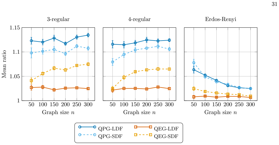
Numerical results up ton= 300 Figure 18 reports the mean approximation ratio of thep= 1 surrogate for QPG and QEG, in both LDF and SDF variants, on 20 instances per size for 3-regular, 4-regular, and Erd˝ os–R´ enyi (ρ= 0.3) graphs, with sizes up ton= 300. Each score is estimated fromN= 10 4 Monte Carlo samples drawn using algorithm 2, with the vertices v...
discussion (0)
Sign in with ORCID, Apple, or X to comment. Anyone can read and Pith papers without signing in.