REVIEW 3 major objections 7 minor 61 references
Structure-preserving Fourier circuits on a trapped-ion processor keep subdomain kinetic-energy dynamics of 1D/2D acoustic waves and variable-mass Dirac evolution within a few percent of classical references at encoded sizes up to 4096.
Reviewed by Pith at T0; open to challenge. T0 means a machine referee read the full paper against a public rubric. the ladder, T0–T4 →
T0 review · grok-4.5
2026-07-31 05:25 UTC pith:CFYMO5PY
load-bearing objection Solid H2-2 hardware benchmark for structured wave PDEs: real size jump and an exact 2D bright–dark block reduction, scoped honestly to low-bandwidth inputs and coarse KE observables. the 3 major comments →
Structure-Preserving Quantum Simulation of Wave Equations on a Trapped-Ion Processor
The pith
A machine-rendered reading of the paper's core claim, the machinery that carries it, and where it could break.
Core claim
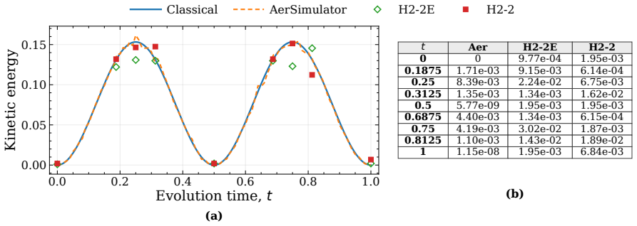
On Quantinuum H2-2, structure-preserving QFT-based circuits for 1D and 2D acoustic waves and Strang-split variable-mass Dirac dynamics produce half-domain kinetic-energy (or related) observables that track classical references with mean absolute errors between 5.9×10^{-3} and 2.4×10^{-2} for encoded state spaces up to 4096, at fixed retained Fourier bandwidth.
What carries the argument
Fourier-block diagonalization via the quantum Fourier transform, plus an exact bright–dark (Morris–Shore) reduction of each 2D acoustic Fourier block that isolates the longitudinal velocity coupled to pressure and removes directional product-formula error; Dirac kinetics and mass are combined by Strang splitting.
Load-bearing premise
The inputs stay on a fixed low Fourier bandwidth so mode angles can be precomputed classically on a small retained set rather than evaluated coherently for broadband fields.
What would settle it
Repeat the same H2-2 kinetic-energy protocol on a broadband or unstructured initial field (or full coherent 2D mode arithmetic without retained-set precomputation) and check whether mean absolute error stays in the reported 10^{-2} range as grid qubits grow.
If this is right
- At fixed retained bandwidth, compiled acoustic gate counts scale roughly quadratically in grid qubits while depth is near-linear in 1D and more quadratic in 2D, and acoustic depth is essentially independent of evolution time.
- Observable-level wave dynamics, not full-state tomography, are a practical NISQ output model for hyperbolic PDEs on trapped-ion hardware.
- The bright–dark block reduction gives an exact alternative to directional Trotterization for constant-coefficient periodic 2D acoustics within each retained Fourier mode.
- Heterogeneous Dirac-type models remain accessible via position–Fourier Strang splitting, at the cost of depth that grows with product-formula steps.
- These benchmarks do not claim quantum advantage over classical PDE solvers; they bound what structured wave observables present hardware can resolve.
Where Pith is reading between the lines
- If low-bandwidth structure is the real enabler, hybrid pipelines that compress classical fields into few Fourier modes before quantum evolution may matter more than raw grid size.
- The same bright–dark idea may transfer to other rank-one pressure–velocity or flux couplings (e.g., simplified elastic or Maxwell blocks) before general sparse encodings are needed.
- Emulator error sometimes exceeding hardware error suggests device-specific calibration, not just gate-count models, should drive next mitigation choices for QFT-heavy wave circuits.
- Scaling beyond retained-mode precomputation will likely be gated first by reversible arithmetic for dispersion and Givens angles, not by the ion-trap connectivity that already suits nonlocal QFTs.
Editorial analysis
A structured set of objections, weighed in public.
Referee Report
Summary. The manuscript constructs and benchmarks structure-preserving Fourier-based quantum circuits for the 1D and 2D acoustic wave equations and a 1D Dirac equation with stepwise mass on Quantinuum H2-2. A Hermitian first-order finite-difference discretization plus QFT reduces 1D acoustics to mode-controlled rotations with a low-mode linearization error bound; 2D acoustics uses an exact bright–dark (Morris–Shore) reduction of each Fourier block that removes directional product-formula error; Dirac dynamics uses Strang splitting between Fourier kinetic and position-space mass terms. Hardware runs reach Nh=1024 (1D) and 32×32 (2D), encoded dimension up to 4096, and report half-domain kinetic-energy (or spinor-population) observables rather than full fields. Across tested cases, H2-2 tracks classical references with MAE between 5.9×10^{-3} and 2.4×10^{-2}. Resource scans show roughly quadratic compiled gate count in nh at fixed retained bandwidth, with acoustic depth essentially t-independent and Dirac cost growing with product-formula steps.
Significance. If the reported hardware agreement and resource scalings hold as stated, this is a meaningful near-term benchmark: it extends prior QFT wave-equation hardware work (notably Wright et al. on H1-1 at nh=6) to nh=10 and to 2D and inhomogeneous Dirac dynamics, introduces an exact bright–dark digital reduction for the constant-coefficient periodic 2D acoustic block, and supplies logical vs H2-2-native gate/depth fits under independent t and nh scans. Strengths include careful structure preservation (Hermitian semi-discrete generators), an explicit low-mode linearization bound O(t K^3/N_h^2), a Strang commutator proposition with bulk/interface split, and transparent classical/Aer/H2-2E/H2-2 comparisons on a physically motivated marginal observable. The authors correctly disclaim quantum advantage and restrict scope to periodic, low-bandwidth inputs and coarse observables. Within that scope the work is a solid hardware-level contribution to quantum PDE simulation.
major comments (3)
- [Abstract, §I, §VII] Abstract and §I/§VII: the headline claim that accurate observable dynamics remain resolvable for structured wave problems with “thousands of encoded degrees of freedom” is only supported under fixed retained Fourier bandwidth (1D linearization §V A 2, Eqs. 35–54; 2D K1={0,±1,±2}, |K|=25, Boolean synthesis §V B 4 and App. B 1, Eqs. B7–B19). The body states this, but the abstract’s resource sentence (“At fixed retained bandwidth…”) is easy to miss relative to the dimension claim. Please elevate one explicit sentence in the abstract (and the concluding claim in §VII) that the nontrivial dynamical support and non-QFT interaction cost are those of a fixed mode set, so the resolvability evidence does not transfer to broadband or unstructured fields without coherent angle evaluation and different depth scaling.
- [§VI C 1, Eq. (128); Prop. V.1] §VI C 1, Eq. (128): the Dirac Strang step schedule r(t) is a hand-tuned staircase (1,2,3,6,7) chosen by classical fidelity sweeps, not derived from the commutator bound in Prop. V.1 / Eq. (115). Because the central Dirac hardware claim (MAE 2.4×10^{-2}, largest in the paper) and the linear-in-t resource fits are tied to this schedule, either (i) report the classical fidelity or ||U−S2^r|| versus r used to select the breakpoints, or (ii) replace/augment with a bound-driven r(t) from CS=∥XA∥+2∥XB∥ for the step mass so readers can separate Trotter error from device error. As written, the t-resource slope mixes algorithmic step growth with compilation in a non-reproducible way.
- [§VI A 2, §VI B 2, §VI C 2; Figs. 3–4, 8–12] §VI A 2 / VI B 2 / VI C 2 and Figs. 3–4, 8–10, 12: hardware MAE is compared to classical references and Aer (8192 shots) while H2-2 uses 1024 shots. For several Gaussian/nonseparable points the H2-2E mean error exceeds H2-2, which the text notes but does not quantify via binomial/shot-noise error bars on ⟨KE⟩. Because the strongest claim is that device errors remain O(10^{-2}) and “track” classical dynamics, add shot-noise uncertainty (or bootstrap intervals) on all hardware and Aer markers and, where MAE is within a few σ of sampling noise, state that explicitly so device noise is not over-attributed.
minor comments (7)
- [Table I] Table I lists this work’s depth as O(log^2 Nh) per step; for Dirac the depth also scales with r(t), and for 2D retained-mode synthesis the prefactor depends on |K|. A footnote clarifying “acoustic, fixed K” versus “Dirac per Strang step” would align the table with §VI.
- [§III B] Eq. (10) and nearby text: “displacenentu” is a typo for “displacement u”.
- [§VI A 1, Fig. 1] Fig. 1 caption and §VI A 1: fits are written with missing signs/spacing in places (e.g. “1.3n2_h + 19.7nh 163.1”); use explicit ± or − for intercepts consistently with the annotated figures.
- [§II] §II: “Suauet al.” and similar missing spaces/italics before “et al.” appear repeatedly; normalize author–et al. spacing.
- [§VI A 2] §VI A 2: “16×16 increase in grid resolution over Wright et al.” for nh=6→10 is a 2^4=16× increase in Nh, not 16×16; rephrase to avoid reading as two-dimensional.
- [§V, Appendix C] Appendix circuit diagrams (Figs. 14–24) are valuable; a single sentence in §V pointing to which figure matches which hardware experiment (cosine/Gaussian/2D/Dirac) would improve navigability.
- [§V B 2, Appendix D] Glossary (Table II) defines N as “system size” and n as total qubits; in the main text N is sometimes used where Nh is meant (e.g. around Eq. 80). Unify Nh versus N.
Circularity Check
No significant circularity: hardware KE comparisons and resource counts are empirical, with classical references and circuit reductions independently derived.
full rationale
The paper’s load-bearing claims are (i) structure-preserving QFT/bright–dark/Strang circuit constructions and (ii) H2-2 measurements of subdomain kinetic energy versus classical references. Classical trajectories are obtained by independent NumPy/SciPy exponentiation of the same semi-discrete Hermitian generators, not by fitting to hardware samples. The 1D low-mode linearization error bound follows from the cubic remainder of sin θ_k; the 2D bright–dark reduction is an algebraic Morris–Shore factorization of each Fourier block (external 1983 structure), removing directional Trotter error by construction of the model rather than by normalizing to measured KE. Resource scalings are compiled gate/depth counts under fixed retained bandwidth—an explicit scope choice, not a fitted parameter renamed as a prediction. Citations to Wright et al. and Lubasch et al. supply prior QFT context; the hardware instances, bright–dark compilation, and Dirac Strang runs are self-contained experiments. Nothing in the derivation chain reduces a claimed prediction to its own inputs by definition or self-citation uniqueness.
Axiom & Free-Parameter Ledger
free parameters (5)
- Retained Fourier set K / K1 =
K1={0,1,2,Nh-2,Nh-1}; cosine often single mode k0=1
- Dirac Strang step schedule r(t) =
r=1,2,3,6,7 on intervals up to t=1
- Gaussian width σ and nonseparable (κ,γ) =
σ=0.2; κ=1.0, γ=0.4
- Mass step (m-, m+) =
m-=0, m+=2 on half-domains
- Hardware shot count =
1024 (device/emulator), 8192 (Aer)
axioms (6)
- domain assumption Periodic finite-difference first-derivative blocks paired with adjoints yield a Hermitian semi-discrete generator, so evolution is unitary on the encoded space.
- standard math Under periodic BCs, circulant difference operators are diagonalized by the QFT, giving independent Fourier-mode blocks.
- domain assumption Smooth initial data are effectively supported on a fixed low-wavenumber band so sin-linearization / retained-mode synthesis errors remain small (bounds Eqs. 51–54, 105–106).
- ad hoc to paper Subdomain kinetic-energy projectors estimated from computational-basis samples are the figure of merit for “accurate observable dynamics.”
- domain assumption Quantinuum H2-2 native compilation via pytket/qnexus and the device noise process are adequately represented by reported gate counts and H2-2 / H2-2E runs.
- domain assumption For noncommuting wave and mass terms, Strang splitting with the chosen r controls the relevant error for the plotted KE trajectories.
invented entities (1)
-
Bright–dark (Morris–Shore) digital reduction of 2D acoustic Fourier blocks
independent evidence
read the original abstract
Wave equations provide a natural testbed for near-term quantum simulation of partial differential equations, but hardware demonstrations have remained limited in spatial dimension, equation class, system size, and physically meaningful output. We develop and benchmark structure-preserving, Fourier-based quantum circuits for the one- and two dimensional acoustic wave equations and Dirac dynamics with variable mass on the Quantinuum H2-2 trapped-ion processor. The experiments include one-dimensional grids with up to \(1024\) points and \(32\times32\) two-dimensional grids, corresponding to an encoded state-space dimension of up to \(4096\). Rather than reconstructing the full fields, we estimate subdomain kinetic energies directly from measurement samples. Across all tested acoustic and Dirac dynamics problems, the H2-2 results track the classical kinetic-energy dynamics with mean absolute errors between \(5.9\times10^{-3}\) and \(2.4\times10^{-2}\). At fixed retained bandwidth, the compiled gate counts grow approximately quadratically with the number of grid qubits; the acoustic circuit sizes are essentially independent of evolution time, whereas the cost also grows with the number of product-formula steps. These results provide hardware-level evidence that accurate observable dynamics can remain resolvable for structured wave problems with thousands of encoded degrees of freedom on a present-day trapped-ion processor.
Figures




Reference graph
Works this paper leans on
-
[1]
Withh= 1/N h and using sinθ k ≥0 for 0≤k < N h, |λk|= 2N h sinθ k, θ k = πk Nh .(29) Thus each block in Eq
Fourier-mode propagator It is convenient to record the modulus ofλ k. Withh= 1/N h and using sinθ k ≥0 for 0≤k < N h, |λk|= 2N h sinθ k, θ k = πk Nh .(29) Thus each block in Eq. (27) simply consists of Pauli operators, Hk =−|λ k| cosθ k σx + sinθ k σy =−|λ k|R z(θk)σ x Rz(−θk).(30) Equivalently, usingσ x = Hσ z H (with H the Hadamard gate), Hk = Rz(θk) H ...
-
[2]
, nh −1}and anyϕ∈R, CR (r) Z (ϕ) = Nh−1X k=0 |k⟩⟨k| ⊗Rz(ϕkr),(39) wherek r ∈ {0,1}is ther-th bit in the binary expansionk= Pnh−1 r=0 kr2r, withN h = 2nh
Low-mode linearization For low Fourier modesk=O(1), we can apply a linear approximation, sin πk Nh ≈ π Nh min(k, Nh −k) = π Nh ks, k s ≡min(k, Nh −k).(35) Substituting this into the diagonal generator of (31) replaces−2N h sinθ k by−2N h · π Nh ks =−2πk s, giving the approximate diagonal generator eHZ = Nh−1X k=0 |k⟩⟨k| ⊗ −2πks σz .(36) For evenN h = 2nh ...
-
[3]
Complete evolution circuit The complete construction for the evolution of the wave equation is given by |Ψ(t)⟩=e −iHt |Ψ(0)⟩(55) H= (F ⊗I)† bH(F ⊗I) =⇒e −iHt = (F † ⊗I) bU(t) (F ⊗I), bU(t) =e −i bHt (56) For the initial conditions considered here, the velocity field vanishes,v(x j,0) = 0, while the flux field is initialized with the non-uniform profilep(x...
-
[4]
(24) to the Fourier domain, we apply the two-dimensional QFT acting on the two spatial registers
Fourier block structure To reduce the Hamiltonian in Eq. (24) to the Fourier domain, we apply the two-dimensional QFT acting on the two spatial registers. F2 =F ⊗ F(60) The transform is applied directly and unconditionally to both registers; no ancillary qubit is needed to choose anx- ory-directional QFT. Specifically, by using Eqs. (23) and (26), we have...
-
[5]
Each of the Hamiltonians is acting in one direction, for which the circuit implemented has been outlined in Section V A
Directional operator splitting A natural approach is to decompose the block into directional couplings, H k =H x(kx) +H y(ky),(67) where Hx =λ x |vx⟩⟨p|+λ ∗ x |p⟩⟨vx|, H y =λ y |vy⟩⟨p|+λ ∗ y |p⟩⟨vy|,(68) and implement them one at a time. Each of the Hamiltonians is acting in one direction, for which the circuit implemented has been outlined in Section V A...
-
[6]
A more efficient construction follows by first identifying the velocity superposition that actually couples to pressure
Bright–dark reduction The directional decomposition treats the two pressure–velocity couplings separately, even though they belong to the same three-state Fourier block. A more efficient construction follows by first identifying the velocity superposition that actually couples to pressure. This is the same algebraic structure that appears in the Morris–Sh...
-
[7]
In the hardware implementation reported here, we do not evaluate the square root or atan2 coherently
Compilation of the nonlinear mode dependence The bright–dark reduction leaves two nonlinear, mode-dependent rotation angles, αk = 2ηk = 2 atan2(Ay, Ax), β k = 2tΩk = 2t q A2x +A 2y.(101) The phasesϕ x andϕ y inP k are simpler because each depends on only one Fourier index. In the hardware implementation reported here, we do not evaluate the square root or...
-
[8]
14 and 15
Resource scaling For the cosine pressure initial state with a single modek 0 = 1, the explicit circuit schematics are given in Figs. 14 and 15. Firstly we study scaling with evolution time, shown in Fig. 1 ([panels (a) and (c)), after transpilation to the native Quantinuum H2-2 gate set corresponding to grid sizeN h = 1024 (n h = 10), the compiled circuit...
2000
-
[9]
S. A. Moseset al., Physical Review X13, 041052 (2023)
2023
-
[10]
Because the full measurement count distribution is available, the kinetic energy can be computed on any subdomain in post-processing; we report the half-domainX= (0, 1 2 ), i.e
Hardware results Rather than reconstructing the velocity and flux fieldsv(x), p(x) at every grid pointx∈(0,1), we evaluate a single physically meaningful observable, the kinetic energy on a subdomainX⊂(0,1). Because the full measurement count distribution is available, the kinetic energy can be computed on any subdomain in post-processing; we report the h...
-
[11]
The detailed circuit construction is described in Section B 2
Resource scaling Similar to the one-dimensional case, we first consider the cosine initial condition for the flux withk x = ky = 1. The detailed circuit construction is described in Section B 2. Further, note that there are only 2 Fourier modes retained in each direction, the Hamiltonian circuit is simplified accordingly. The resource estimation here foll...
2048
-
[12]
In the field encoding of Eq
Hardware results As in Section VI A 2, we evaluate a single physically meaningful observable rather than reconstructing the full field: the kinetic energy carried by thev x component on a spatial subdomainx∈[0,1/2). In the field encoding of Eq. (65),v x corresponds to both field qubit state being|00⟩, so ⟨KEvx ⟩=I y ⊗ |0⟩ ⟨0|M SBx ⊗I nh−1 ⊗ |00⟩⟨00|f ,(12...
-
[13]
The simulations have been done for grid-size ofN h = 32(nh = 5) corresponding to total system ofn= 12 qubits. For the cosine intial pressure, the mean absolute error averaged over its sampled points is 2.8×10 −3 for AerSimulator, 9.8×10 −3 for H2-2E, and 7.9×10 −3 for H2-2 - the same ordering, and similar∼3× increase from the shot-noise reference to hardw...
2000
-
[14]
(122) with m− = 0,m + = 2, and, following the same protocol as Section VI A 1
Resource scaling For the cosine pressure initial state, we takek 0 = 1 and the step-function mass profile of Eq. (122) with m− = 0,m + = 2, and, following the same protocol as Section VI A 1. Because the Trotter step countr=t/τ in Eq. (107) must grow withtto control the localτ 3 error, our implementation uses a coarse step schedule or Trotter number given...
-
[15]
(123), since the Dirac-dynamics circuit retains the one-dimensional construction’s velocity–flux field encoding with the mass term added only through the TrotterizedH mass sub-step
Hardware results We evaluate the same kinetic-energy observable as in Section VI A 2, Eq. (123), since the Dirac-dynamics circuit retains the one-dimensional construction’s velocity–flux field encoding with the mass term added only through the TrotterizedH mass sub-step. Figure 12 shows the resulting kinetic energy as a function of evolution time. 0.0 0.2...
-
[16]
It therefore suffices to prepare|ψ p⟩in the spatial register
Initial-state preparation We restrict attention to initial conditions with vanishing velocity,v(x,0) = 0, so that the complete initial state factorizes as |Ψ(0)⟩=|ψ p⟩ |p⟩,(A1) where|ψ p⟩carries the Fourier coefficients of the initial pressure field and|p⟩is the field register. It therefore suffices to prepare|ψ p⟩in the spatial register. We give two cons...
-
[17]
This case is small enough that the nonlinear angles can be synthesized by Boolean expansions in the retained-mode bits, avoiding a general arithmetic circuit
Explicit synthesis for the retained low-mode set We now specialize to the retained one-dimensional mode set K1 ={0,1,2, N h −2, Nh −1}.(B1) The two-dimensional retained set isK=K 1 × K1. This case is small enough that the nonlinear angles can be synthesized by Boolean expansions in the retained-mode bits, avoiding a general arithmetic circuit. a. Sign-mag...
-
[18]
Preparation of two-dimensional flux states We finally describe the preparation of the Fourier-space flux state used as input to the circuit. For a pressure-only initial conditionv x(x, y,0) =vy(x, y,0) = 0, the initial Fourier state has the form |Ψf (0)⟩=|ψ f ⟩xy |p⟩,|ψ f ⟩xy = Nh−1X kx,ky=0 bfkx,ky |kx⟩x |ky⟩y .(B20) If the initial data are prepared in p...
-
[19]
R. P. Feynman, International Journal of Theoretical Physics21, 467 (1982)
1982
-
[20]
Lloyd, Science273, 1073 (1996)
S. Lloyd, Science273, 1073 (1996)
1996
-
[21]
D. W. Berry, Journal of Physics A: Mathematical and Theoretical47, 105301 (2014), arXiv:1010.2745
Pith/arXiv arXiv 2014
-
[22]
A. W. Harrow, A. Hassidim, and S. Lloyd, Physical Review Letters103, 150502 (2009), arXiv:0811.3171
Pith/arXiv arXiv 2009
-
[23]
Preskill, Quantum2, 79 (2018), arXiv:1801.00862
J. Preskill, Quantum2, 79 (2018), arXiv:1801.00862
Pith/arXiv arXiv 2018
-
[24]
A. C. Hughes, R. Srinivas, C. M. L¨ oschnauer, H. M. Knaack, R. Matt, C. J. Ballance, M. Malinowski, T. P. Harty, and R. T. Sutherland, Trapped-ion two-qubit gates with>99.99% fidelity without ground-state cooling (2025), arXiv:2510.17286 [quant-ph]
arXiv 2025
-
[25]
Marxer, J
F. Marxer, J. Mro˙ zek, J. Andersson, L. Abdurakhimov, J. Adam, V. Bergholm, R. Beriwal, C. F. Chan, S. Dahl, S. R. Das, F. Deppe, O. Fedorets, Z. Gao, A. Gomez Frieiro, D. Gusenkova, A. Guthrie, T. Hiltunen, H. Hsu, E. Hyypp¨ a, J. Ikonen, S. Inel, S. W. Jolin, A. Karis, S.-G. Kim, W. Kindel, A. Komlev, M. Koistinen, R. Kokkoniemi, S. Kumar, H.-S. Ku, J....
2026
-
[26]
Wen and Y
X. Wen and Y. Wang, Journal of Geophysical Research: Machine Learning and Computation2, e2024JH000473 (2025)
2025
-
[27]
Babbush, N
R. Babbush, N. Wiebe, J. McClean, J. McClain, H. Neven, and G. K.-L. Chan, Physical Review X8, 011044 (2018)
2018
-
[28]
L. Wright, C. Mc Keever, J. T. First, R. Johnston, J. Tillay, S. Chaney, M. Rosenkranz, and M. Lubasch, Physical Review Research6, 043169 (2024), arXiv:2402.19247
Pith/arXiv arXiv 2024
-
[29]
Lubasch, Y
M. Lubasch, Y. Kikuchi, L. Wright, and C. Mc Keever, Physical Review Research7, 043326 (2025)
2025
-
[30]
J. R. Morris and B. W. Shore, Physical Review A27, 906 (1983)
1983
-
[31]
R. G. Unanyan, J. Otterbach, M. Fleischhauer, J. Ruseckas, V. Kudriaˇ sov, and G. Juzeli¯ unas, Physical Review Letters105, 173603 (2010)
2010
-
[32]
P. C. S. Costa, S. Jordan, and A. Ostrander, Physical Review A99, 012323 (2019), arXiv:1711.05394. 43
Pith/arXiv arXiv 2019
-
[33]
A. Suau, G. Staffelbach, and H. Calandra, ACM Transactions on Quantum Computing2, 1 (2021), arXiv:2003.12458
Pith/arXiv arXiv 2021
-
[34]
A. M. Childs, J.-P. Liu, and A. Ostrander, Quantum5, 574 (2021), arXiv:2002.07868
Pith/arXiv arXiv 2021
-
[35]
Y. Sato, R. Kondo, I. Hamamura, T. Onodera, and N. Yamamoto, Physical Review Research6, 033246 (2024), arXiv:2402.18398
Pith/arXiv arXiv 2024
-
[36]
B. Arseniev, D. Guskov, R. Sengupta, and I. Zacharov, High order schemes for solving partial differential equa- tions on a quantum computer (2024), arXiv:2412.19232 [quant-ph]
Pith/arXiv arXiv 2024
-
[37]
M. Schade, C. B¨ osch, V. Hapla, and A. Fichtner, Geophysical Journal International238, 321 (2024), arXiv:2312.14747
Pith/arXiv arXiv 2024
-
[38]
B. Zanger, C. B. Mendl, M. Schulz, and M. Schreiber, Quantum5, 502 (2021), arXiv:2012.09469
Pith/arXiv arXiv 2021
-
[39]
Schillo and A
N. Schillo and A. Sturm, IEEE Transactions on Quantum Engineering6, 3100416 (2025)
2025
-
[40]
R. Gerritsma, G. Kirchmair, F. Z¨ ahringer, E. Solano, R. Blatt, and C. F. Roos, Nature463, 68 (2010), arXiv:0909.0674
Pith/arXiv arXiv 2010
-
[41]
R. Gerritsma, B. P. Lanyon, G. Kirchmair, F. Z¨ ahringer, C. Hempel, J. Casanova, J. J. Garc ´ ıa-Ripoll, E. Solano, R. Blatt, and C. F. Roos, Physical Review Letters106, 060503 (2011), arXiv:1007.3683
Pith/arXiv arXiv 2011
-
[42]
M. Kapil, B. K. Behera, and P. K. Panigrahi, Quantum simulation of Klein Gordon equation and observation of Klein paradox in IBM quantum computer (2018), arXiv:1807.00521 [quant-ph]
Pith/arXiv arXiv 2018
-
[43]
Larsson and V
S. Larsson and V. Thom´ ee,Partial Differential Equations with Numerical Methods, 1st ed., Texts in Applied Mathematics, Vol. 45 (Springer Berlin, Heidelberg, 2003)
2003
-
[44]
G. A. Baker, SIAM Journal on Numerical Analysis13, 564 (1976)
1976
-
[46]
S. Jin, X. Li, and N. Liu, Quantum6, 739 (2022)
2022
-
[47]
A. Javadi-Abhari, M. Treinish, K. Krsulich, C. J. Wood, J. Lishman, J. Gacon, S. Martiel, P. D. Nation, L. S. Bishop, A. W. Cross, B. R. Johnson, and J. M. Gambetta, Quantum computing with Qiskit (2024), arXiv:2405.08810 [quant-ph]
Pith/arXiv arXiv 2024
-
[48]
S. Sivarajah, S. Dilkes, A. Cowtan, W. Simmons, A. Edgington, and R. Duncan, Quantum Science and Technology 6, 014003 (2020), arXiv:2003.10611
Pith/arXiv arXiv 2020
-
[49]
Quantinuum, Quantinuum nexus,https://nexus.quantinuum.com/(2024), accessed July 25, 2026
2024
-
[50]
Fleischhauer, A
M. Fleischhauer, A. Imamoglu, and J. P. Marangos, Reviews of Modern Physics77, 633 (2005)
2005
-
[51]
B. T. Torosov and N. V. Vitanov, Physical Review Research2, 043194 (2020)
2020
-
[52]
I. F. Araujo, C. Blank, I. C. S. Ara´ ujo, and A. J. da Silva, IEEE Transactions on Computer-Aided Design of Integrated Circuits and Systems43, 161 (2024)
2024
-
[53]
K. Temme, S. Bravyi, and J. M. Gambetta, Physical Review Letters119, 10.1103/physrevlett.119.180509 (2017)
-
[54]
N. Ezzell, B. Pokharel, L. Tewala, G. Quiroz, and D. A. Lidar, Physical Review Applied20, 10.1103/physrevap- plied.20.064027 (2023)
-
[55]
W. M. Watkins, L. M. Norris, R. Hutson, M. Urmey, P. Siegfried, and C. H. Baldwin, Improving dynamical decoupling for trapped-ion qccd quantum computers (2026), arXiv:2607.14441 [quant-ph]
Pith/arXiv arXiv 2026
-
[56]
Z. Cai, R. Babbush, S. C. Benjamin, S. Endo, W. J. Huggins, Y. Li, J. R. McClean, and T. E. O’Brien, Reviews of Modern Physics95, 10.1103/revmodphys.95.045005 (2023)
-
[57]
C. N. Self, M. Benedetti, and D. Amaro, Nature Physics20, 219–224 (2024)
2024
-
[58]
M. A. Perlin, Z. He, A. A. Armenakas, P. Andres-Martinez, T. Hao, D. Herman, Y. Jin, K. Mayer, C. Self, D. Amaro, C. Ryan-Anderson, and R. Shaydulin, Fault-tolerant execution of error-corrected quantum algorithms (2026), arXiv:2603.04584 [quant-ph]
arXiv 2026
-
[59]
F. B. Maciejewski, Z. Zimbor´ as, and M. Oszmaniec, Quantum4, 257 (2020)
2020
-
[60]
Y. Xu, K. Zhao, H.-T. Liu, K. Huang, Z. Liu, H. Fan, and H. Hu, Journal of the Mechanics and Physics of Solids 213, 106639 (2026)
2026
-
[61]
S. Jin, N. Liu, and C. Ma, ESAIM: Mathematical Modelling and Numerical Analysis58, 1853 (2024). 44
2024
-
[73]
These results confirm that QFT allows the wave dynamics can be simulated at almost constant depth, due to the fast-forwarding by QFT
at these times. These results confirm that QFT allows the wave dynamics can be simulated at almost constant depth, due to the fast-forwarding by QFT. Next, we examine the scaling with grid size with results shown in Fig. 1 ([panels (b) and (d)). At the fixed timet= 0.1 we scan the register size overn h ∈ {6,10,14, . . . ,50}, in order to capture asymptoti...
2000
discussion (0)
Sign in with ORCID, Apple, or X to comment. Anyone can read and Pith papers without signing in.