REVIEW 3 major objections 5 minor 56 references
A pipeline with zero learned parameters rivals trained LiDAR scene-flow networks—and holds up best at long range.
Reviewed by Pith at T0; open to challenge. T0 means a machine referee read the full paper against a public rubric. the ladder, T0–T4 →
T0 review · deepseek-v4-flash
2026-08-03 11:01 UTC pith:S773P2NM
load-bearing objection A serious training-free scene flow baseline that deserves referee time, but the long-range headline oversells the actual ranking and the challenge result is hard to audit without code. the 3 major comments →
CorrelationFlow: A Training-Free Geometric Approach for LiDAR Scene Flow Estimation
The pith
A machine-rendered reading of the paper's core claim, the machinery that carries it, and where it could break.
Core claim
The paper's central claim is that scene flow estimation reduces to two textbook operations: connected-component labeling and correlation maximization on bird's-eye-view occupancy images. The dense variant aggregates ego-motion-compensated sweeps into one binary image, extracts spatio-temporal connected components as object hypotheses, and estimates each component's flow as the pixel shift that maximizes normalized cross-correlation between its footprints; the keypoint variant drops clustering and matches boundary-patch descriptors on a single sweep pair, then densifies under the rigidity prior. Because nothing is trained, nothing is inherited: on a five-dataset benchmark with heterogeneous s
What carries the argument
The load-bearing object is the binary bird's-eye-view occupancy image built from ego-motion-compensated LiDAR sweeps at 0.1 m resolution. On it sit two mechanisms: spatio-temporal connected components—found by dilating the aggregated image and labeling connected foreground regions, with a size-based validation split that re-splits over-large components—provide object hypotheses whose pixels share one rigid horizontal translation; normalized cross-correlation (NCC) scores how well the template footprint at time t fits each placement at time t+1, so the correlation peak directly gives the flow vector. Supporting machinery: median pooling over past baselines, coarse-to-fine warping, and, in the
Load-bearing premise
The approach stands or falls on the assumption that, after ego-motion compensation, connected components of the dilated BEV image correspond one-to-one to physical objects translating rigidly; if a merge or split occurs, the error propagates directly into the recovered flow, and the paper itself notes this is exactly what happens for sparse, distant, and crowded scenes.
What would settle it
Take a scene with two stationary objects parked 1–2 m apart and record their 3D point clouds; if connected-component clustering merges them into one component (as the 0.1 m pixel plus 3×3 dilation would tend to do at close gaps) and assigns both objects a nonzero flow because the NCC peak locks onto one footprint, the central premise fails. A second check: on crowded 35–70 m scenes, compute the under-segmentation rate against instance labels; high merge rates would undermine the claimed long-range advantage.
If this is right
- A zero-parameter estimator can serve as a reproducible yardstick: any learned method that cannot beat connected-component clustering plus correlation on the Dynamic Bucket-Normalized EPE is adding parameters without adding insight.
- The 35–70 m robustness follows from aggregating evidence over entire object footprints, so scene flow evaluation should weight long-range and sparse-object errors explicitly rather than averaging over mostly short-range dense points.
- Because connected-component clustering on a fixed BEV grid has complexity independent of point count, a near-real-time path exists for training-free flow, unlike density clustering whose cost grows with sweep size.
- The keypoint variant's single-sweep operation—nearly matching the dense method's best temporal-window configuration—means flow can be computed from one sweep pair where history is unavailable, such as the first frames of a sequence.
Where Pith is reading between the lines
- I infer the strongest test of the paper's thesis is a hybrid: using CorrelationFlow's footprint-level flow as initialization or verification for learned per-point refiners; if the geometric prior already captures most motion, the learned component should only need to correct residual rotation and articulation.
- I infer the method's reliance on planar, translation-only motion means it would degrade predictably on steep slopes or articulated objects such as a person with swinging limbs; a testable extension is multi-height occupancy slices to recover vertical motion without the sectional view.
- I infer the benchmark's Dynamic Bucket-Normalized EPE may under-reward absolute accuracy at long range, and that a per-range breakdown should become standard reporting practice; the paper's own range analysis suggests the ranking of learned baselines reverses under this lens.
- A direct extension would replace the binary occupancy image with intensity- or reflectivity-weighted occupancy, giving the correlation a sharper peak for textureless footprints; whether this helps or hurts at long range is a cheap experiment the paper does not run.
Editorial analysis
A structured set of objections, weighed in public.
Referee Report
Summary. The paper proposes CorrelationFlow, a fully training-free LiDAR scene flow estimator. Consecutive ego-motion-compensated sweeps are projected to bird's-eye-view (BEV) occupancy images; spatio-temporal connected components identify objects; and each component's horizontal translation is estimated as the peak of normalized cross-correlation between its BEV footprints. The flow is propagated to all member points. A sparse variant, CorrelationFlow-Keypoints, matches boundary descriptors on a single sweep pair and densifies via connected components. The method is evaluated on the Argoverse 2 2026 Multi-Dataset Scene Flow Challenge using Dynamic Bucket-Normalized EPE, where it reportedly ranks second among unsupervised methods and degrades less than learned baselines at 35–70 m range. Ablations examine pixel size, an optional sectional view, clustering method, temporal window size, multi-scale refinement, and keypoint densification.
Significance. If the reported results are reproducible, this is a valuable counterpoint to the learned-scene-flow monoculture: the paper shows that a zero-parameter pipeline built from connected components and correlation can be competitive across five heterogeneous datasets. The manuscript is honest in its ablations, including the admission that HDBSCAN gives better accuracy than the proposed connected-component clustering in the base comparison, that pedestrians remain the weak class, and that the sectional view adds little on flat ground. The lack of training and the validation-split hyperparameter selection are genuine strengths. The central long-range claim is plausible but needs sharper evidence, as discussed below. Overall the contribution is real, but the manuscript currently leaves reproducibility and some interpretive details unresolved.
major comments (3)
- [Sec. VI / final configuration] The exact configuration used for the challenge test is never stated. The ablation fixes pixel size s=0.1 m (Table I), but the final values of the number of past sweeps h, the number of coarse-to-fine scales, the component validation threshold d_max, the Lowe ratio ρ, the descriptor patch size L, and the keypoint gating radius mentioned in Sec. VII are not reported. Without these values, the main performance claim cannot be reproduced and the 'no per-dataset tuning' assertion is not auditable. Please provide a complete hyperparameter table and, if possible, code release.
- [Sec. VI-A / Table III] The connected-component clustering is presented as a contribution, but Table III shows that replacing it with HDBSCAN in the otherwise identical pipeline reduces mean Dynamic Bucket-Normalized EPE from 0.3524 to 0.3247 (7.8% improvement). The paper argues that the proposed clustering improves with past sweeps, but Table III is evaluated without the temporal window; no HDBSCAN + past-sweep + multi-scale ablation is provided. Thus the claim that the proposed clustering is a generally 'density-robust' grouping strategy is not supported by the data. Please report the same pipeline with h>0 and multiple scales for both clustering methods, or revise the claim to emphasize speed and parameter-lightness rather than accuracy.
- [Sec. VI-B / Fig. 12] The abstract's central claim is that CorrelationFlow 'degrades most gracefully at long range—where the shared assumptions of learned methods break down.' Fig. 12 supports this with two range bins, but the metric definition in Sec. VI is ambiguous on whether static points are included: the paper says Dynamic Bucket-Normalized EPE normalizes 'the error for dynamic points,' which would already exclude the static-background zero-flow confound. Please state explicitly whether static points are part of this metric; if they are excluded, say so in the caption and the text, because that directly addresses the static-vs-dynamic concern. If they are included, report a static/dynamic split. In either case, a per-class range breakdown (CAR / OTHER / PED / VRU) would show whether the long-range advantage is concentrated in a particular moving-object class, which is what the 'shared assumptions' claim
minor comments (5)
- [Eq. (1)] The pose notation T^E_t with the description 'pose of the ego vehicle with respect to the global frame' is confusing: normally one would write T_W^t or T_E^t with explicit source/target frames. Please clarify the convention and verify that Eq. (1) maps points from the time-t ego frame to the time-(t+1) ego frame as intended.
- [Sec. VI-B] The baselines 'SeFlow++ [?]' and 'RVLoss [?]' have placeholder citation markers. These must be filled with proper references before submission.
- [Sec. VII] The keypoint variant is said to depend on the 'gating radius,' but this quantity is never defined in Sec. V. Define it or remove the reference.
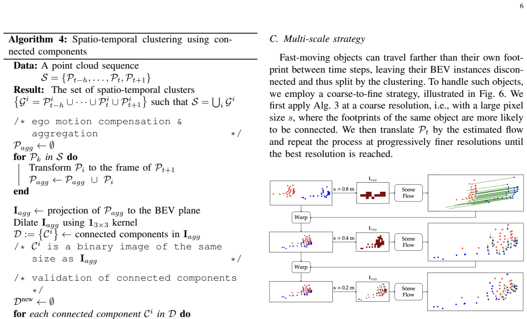
- [Algorithm 4] In the ego-motion compensation step, the loop variable is P_k but the text says 'Transform P_i to the frame of P_{t+1}.' This is a typo and should be corrected.
- [Figs. 9 and 10] The ablation plots show no error bars or repeated-run variability. Since the validation split is a single dataset, at least describe the expected variance or report per-sequence statistics.
Circularity Check
No significant circularity: the derivation is self-contained, hyperparameters are tuned on validation and evaluated on a held-out multi-dataset test set.
full rationale
CorrelationFlow's pipeline is training-free and derives each cluster's flow from the argmax of normalized cross-correlation between BEV occupancy images (Eqs. 5-6 and Algorithm 1); no ground-truth flow is used to fit the method, so no fitted quantity is later relabeled as a prediction. The hyperparameters (pixel size, number of past sweeps, scale count) are chosen on the Argoverse 2 validation split (Table I, Figs. 9-10) and then applied to the held-out five-dataset challenge test set, a clean and disclosed separation. The rigid-planar-motion and footprint-connectivity assumptions are stated explicitly in Secs. III and IV and revisited in the limitations (Sec. VII); they are premises of the method, not conclusions imported through citation. Citations to the authors' own prior work (ICP-Flow [31], VoteFlow [21]) are contextual related-work references and do not carry the derivation. The absence of a static/dynamic decomposition in the long-range analysis of Fig. 12 is a possible validity concern for the 'most graceful degradation' claim, but it concerns benchmark interpretation rather than circular identity between input and output. No load-bearing step reduces, by the paper's own equations or by self-citation, to its own inputs.
Axiom & Free-Parameter Ledger
free parameters (7)
- BEV pixel size s =
0.1 m
- Number of past sweeps h =
4
- Number of coarse-to-fine scales =
not stated for final configuration
- Component validation threshold d_max =
not stated
- Lowe ratio threshold rho =
not stated (rho > 1)
- Descriptor patch size L =
not stated (odd integer)
- Keypoint gating radius =
not stated
axioms (6)
- domain assumption Ego-motion poses T^E_t used in Eq. (1) are accurate.
- domain assumption Objects move rigidly and predominantly planar, with negligible inter-frame rotation.
- domain assumption Constant velocity across the pooled sweep window.
- domain assumption Ego-compensated BEV footprints of one object are connected across consecutive time steps, so connected components map to objects.
- domain assumption The quantized best-overlap translation approximates the true projected displacement.
- standard math Standard algorithmic results are valid: connected-component labeling (Bolelli et al. 2022), distance transform (Borgefors 1986), fast NCC (Lewis 1995), Lowe's ratio test (Lowe 2004).
read the original abstract
LiDAR scene flow estimation has settled into a monoculture: nearly all recent methods share the same feed-forward architecture and the same family of self-supervised losses, inheriting each other's assumptions, and each other's blind spots. When those assumptions fail, as they do for sparse, distant, or fast-moving objects, every method built on them fails together, and adding parameters or simulated training data does not fix what the formulation itself gets wrong. This paper takes the opposite path. We present CorrelationFlow, a training-free geometric framework that reduces scene flow to two textbook operations: connected-component labeling and correlation maximization on bird's-eye-view occupancy images. Objects are isolated as spatio-temporal connected components, their motions recovered as correlation peaks, and the resulting velocities propagated to all member points. However, this dense correlation evaluates every candidate displacement of every cluster and requires a window of past sweeps; therefore, we develop a sparse counterpart that operates on a single sweep pair by matching lightweight occupancy descriptors at boundary key points. Because nothing is trained, nothing is inherited: on the multi-domain test set of the Argoverse 2 2026 Scene Flow Challenge, spanning five datasets with heterogeneous sensors and platforms, CorrelationFlow ranked second among unsupervised methods and degrades most gracefully at long range, where the shared assumptions of learned methods break down. Our results suggest that a substantial share of the scene flow problem is solvable by classical computer vision, and that progress may require questioning the formulation, not scaling it.
Figures




Reference graph
Works this paper leans on
-
[1]
Three- dimensional scene flow,
S. Vedula, S. Baker, P. Rander, R. Collins, and T. Kanade, “Three- dimensional scene flow,” inProceedings of the Seventh IEEE Interna- tional Conference on Computer Vision, vol. 2, 1999, pp. 722–729 vol.2
1999
-
[2]
UNION: Unsupervised 3D object detection using object appearance-based pseudo-classes,
T. Lentsch, H. Caesar, and D. M. Gavrila, “UNION: Unsupervised 3D object detection using object appearance-based pseudo-classes,” in Advances in Neural Information Processing Systems (NeurIPS), vol. 37, 2024, pp. 22 028–22 046
2024
-
[3]
Motion inspired unsupervised perception and prediction in autonomous driving,
M. Najibi, J. Ji, Y . Zhou, C. R. Qi, X. Yan, S. Ettinger, and D. Anguelov, “Motion inspired unsupervised perception and prediction in autonomous driving,” inEuropean Conference on Computer Vision. Springer, 2022, pp. 424–443
2022
-
[4]
Flow-guided motion prediction with semantics and dynamic occupancy grid maps,
R. Asghar, W. Liu, L. Rummelhard, A. Spalanzani, and C. Laugier, “Flow-guided motion prediction with semantics and dynamic occupancy grid maps,” in2024 IEEE 27th International Conference on Intelligent Transportation Systems (ITSC). IEEE, 2024, pp. 3160–3165
2024
-
[5]
Flownet3d: Learning scene flow in 3d point clouds,
X. Liu, C. R. Qi, and L. J. Guibas, “Flownet3d: Learning scene flow in 3d point clouds,”CVPR, 2019
2019
-
[6]
Scalable scene flow from point clouds in the real world,
P. Jund, C. Sweeney, N. Abdo, Z. Chen, and J. Shlens, “Scalable scene flow from point clouds in the real world,”IEEE Robotics and Automation Letters, vol. 7, no. 2, pp. 1589–1596, 2021
2021
-
[7]
DeFlow: Decoder of scene flow network in autonomous driving,
Q. Zhang, Y . Yang, H. Fang, R. Geng, and P. Jensfelt, “DeFlow: Decoder of scene flow network in autonomous driving,” in2024 IEEE International Conference on Robotics and Automation (ICRA), 2024, pp. 2105–2111
2024
-
[8]
Flow4d: Leveraging 4d voxel network for lidar scene flow estimation,
J. Kim, J. Woo, U. Shin, J. Oh, and S. Im, “Flow4d: Leveraging 4d voxel network for lidar scene flow estimation,”IEEE Robotics and Automation Letters, vol. 10, no. 4, pp. 3462–3469, 2025
2025
-
[9]
Neural scene flow prior,
X. Li, J. Kaesemodel Pontes, and S. Lucey, “Neural scene flow prior,” Advances in Neural Information Processing Systems, vol. 34, 2021
2021
-
[10]
ZeroFlow: Fast Zero Label Scene Flow via Distillation,
K. Vedder, N. Peri, N. Chodosh, I. Khatri, E. Eaton, D. Jayaraman, Y . L. D. Ramanan, and J. Hays, “ZeroFlow: Fast Zero Label Scene Flow via Distillation,”International Conference on Learning Representations (ICLR), 2024
2024
-
[11]
Re-evaluating lidar scene flow,
N. Chodosh, D. Ramanan, and S. Lucey, “Re-evaluating lidar scene flow,” in2024 IEEE/CVF Winter Conference on Applications of Com- puter Vision (WACV), 2024, pp. 5993–6003
2024
-
[12]
I can’t believe it’s not scene flow!
I. Khatri, K. Vedder, N. Peri, D. Ramanan, and J. Hays, “I can’t believe it’s not scene flow!” inComputer Vision – ECCV 2024: 18th European Conference, Milan, Italy, September 29 – October 4, 2024, Proceedings, Part XVIII. Berlin, Heidelberg: Springer-Verlag, 2024, p. 242–257. [Online]. Available: https://doi.org/10.1007/978-3-031-72649-1_14
-
[13]
Pointflownet: Learning representations for rigid motion estimation from point clouds,
A. Behl, D. Paschalidou, S. Donné, and A. Geiger, “Pointflownet: Learning representations for rigid motion estimation from point clouds,” inCVPR, 2019
2019
-
[14]
Hplflownet: Hierarchical permutohedral lattice flownet for scene flow estimation on large-scale point clouds,
X. Gu, Y . Wang, C. Wu, Y . J. Lee, and P. Wang, “Hplflownet: Hierarchical permutohedral lattice flownet for scene flow estimation on large-scale point clouds,” inComputer Vision and Pattern Recognition (CVPR), 2019 IEEE International Conference on, 2019
2019
-
[15]
Pointpwc-net: Cost volume on point clouds for (self-) supervised scene flow estimation,
W. Wu, Z. Y . Wang, Z. Li, W. Liu, and L. Fuxin, “Pointpwc-net: Cost volume on point clouds for (self-) supervised scene flow estimation,” in European Conference on Computer Vision. Springer, 2020, pp. 88–107
2020
-
[16]
Scalable scene flow from point clouds in the real world,
P. Jund, C. Sweeney, N. Abdo, Z. Chen, and J. Shlens, “Scalable scene flow from point clouds in the real world,”IEEE Robotics and Automation Letters, vol. 7, no. 2, pp. 1589–1596, 2022
2022
-
[17]
Dynamic 3d scene analysis by point cloud accumulation,
S. Huang, Z. Gojcic, J. Huang, A. Wieser, and K. Schindler, “Dynamic 3d scene analysis by point cloud accumulation,” inECCV, 2022
2022
-
[18]
Deltaflow: An efficient multi-frame scene flow estimation method,
Q. Zhang, X. Zhu, Y . Zhang, Y . Cai, O. Andersson, and P. Jensfelt, “Deltaflow: An efficient multi-frame scene flow estimation method,” in NeurIPS, 2025
2025
-
[19]
Slim: Self-supervised lidar scene flow and motion segmentation,
S. Andreas Baur, D. Josef Emmerichs, F. Moosmann, P. Pinggera, B. Ommer, and A. Geiger, “Slim: Self-supervised lidar scene flow and motion segmentation,” in2021 IEEE/CVF International Conference on Computer Vision (ICCV), 2021, pp. 13 106–13 116
2021
-
[20]
Just go with the flow: Self-supervised scene flow estimation,
H. Mittal, B. Okorn, and D. Held, “Just go with the flow: Self-supervised scene flow estimation,” inCVPR, 2020
2020
-
[21]
V oteflow: Enforcing local rigidity in self-supervised scene flow,
Y . Lin, S. Wang, L. Nan, J. Kooij, and H. Caesar, “V oteflow: Enforcing local rigidity in self-supervised scene flow,” inProceedings of the Computer Vision and Pattern Recognition Conference, 2025, pp. 17 155– 17 164
2025
-
[22]
TeFlow: Enabling multi-frame supervision for self- supervised feed-forward scene flow estimation,
Q. Zhang, C. Jiang, X. Zhu, Y . Miao, Y . Zhang, O. Andersson, and P. Jensfelt, “TeFlow: Enabling multi-frame supervision for self- supervised feed-forward scene flow estimation,” inCVPR, 2026
2026
-
[23]
Seflow: A self-supervised scene flow method in autonomous driving,
Q. Zhang, Y . Yang, P. Li, O. Andersson, and P. Jensfelt, “Seflow: A self-supervised scene flow method in autonomous driving,” inEuropean Conference on Computer Vision. Springer, 2024, pp. 353–369
2024
-
[24]
Deformation and cor- respondence aware unsupervised synthetic-to-real scene flow estimation for point clouds,
Z. Jin, Y . Lei, N. Akhtar, H. Li, and M. Hayat, “Deformation and cor- respondence aware unsupervised synthetic-to-real scene flow estimation for point clouds,” inCVPR, 2022
2022
-
[25]
Synflow: Scaling up lidar scene flow estimation with synthetic data,
Q. Zhang, X. Zhu, C. Jiang, and P. Jensfelt, “Synflow: Scaling up lidar scene flow estimation with synthetic data,”arXiv preprint arXiv:2604.09411, 2026. 12 0-35m 35-70m0.1 0.3 0.5 0.7 0.9 Dynamic Bucket-Normalized EPE AEV A CorrelationFlow SSF CorrelationFlow-Keypoint RVLoss TeFlow SeFlow++ V oteFlow SeFlow 0-35m 35-70m0.1 0.3 0.5 0.7 0.9 A V2 0-35m 35-7...
Pith/arXiv arXiv 2026
-
[26]
Neural eulerian scene flow fields,
K. Vedder, N. Peri, I. Khatri, S. Li, E. Eaton, M. Kocamaz, Y . Wang, Z. Yu, D. Ramanan, and J. Pehserl, “Neural eulerian scene flow fields,” inICLR, 2025
2025
-
[27]
Floxels: Fast unsupervised voxel based scene flow estimation,
D. T. Hoffmann, S. H. Raza, H. Jiang, D. Tananaev, S. Klingenhoefer, and M. Meinke, “Floxels: Fast unsupervised voxel based scene flow estimation,” inProceedings of the IEEE/CVF Conference on Computer Vision and Pattern Recognition, 2025, pp. 22 328–22 337
2025
-
[28]
Rigid scene flow for 3d lidar scans,
A. Dewan, T. Caselitz, G. D. Tipaldi, and W. Burgard, “Rigid scene flow for 3d lidar scans,” in2016 IEEE/RSJ International Conference on Intelligent Robots and Systems (IROS), 2016, pp. 1765–1770
2016
-
[29]
Weakly supervised learning of rigid 3d scene flow,
Z. Gojcic, O. Litany, A. Wieser, L. J. Guibas, and T. Birdal, “Weakly supervised learning of rigid 3d scene flow,” inProceedings of the IEEE/CVF Conference on Computer Vision and Pattern Recognition (CVPR), 2021, pp. 5692–5703
2021
-
[30]
Rigidflow: Self- supervised scene flow learning on point clouds by local rigidity prior,
R. Li, C. Zhang, G. Lin, Z. Wang, and C. Shen, “Rigidflow: Self- supervised scene flow learning on point clouds by local rigidity prior,” inCVPR, 2022
2022
-
[31]
ICP-Flow: Lidar scene flow estimation with icp,
Y . Lin and H. Caesar, “ICP-Flow: Lidar scene flow estimation with icp,” inCVPR, 2024
2024
-
[32]
Density-based clustering based on hierarchical density estimates,
R. J. Campello, D. Moulavi, and J. Sander, “Density-based clustering based on hierarchical density estimates,” inPacific-Asia conference on knowledge discovery and data mining, 2013
2013
-
[33]
hdbscan: Hierarchical density based clustering,
L. McInnes, J. Healy, and S. Astels, “hdbscan: Hierarchical density based clustering,”The Journal of Open Source Software, 2017
2017
-
[34]
Pv-raft: Point-voxel corre- lation fields for scene flow estimation of point clouds,
Y . Wei, Z. Wang, Y . Rao, J. Lu, and J. Zhou, “Pv-raft: Point-voxel corre- lation fields for scene flow estimation of point clouds,” inProceedings of the IEEE/CVF conference on computer vision and pattern recognition, 2021, pp. 6954–6963
2021
-
[35]
Visual object tracking using adaptive correlation filters,
D. S. Bolme, J. R. Beveridge, B. A. Draper, and Y . M. Lui, “Visual object tracking using adaptive correlation filters,” inProceedings of the IEEE Computer Society Conference on Computer Vision and Pattern Recognition (CVPR), 2010, pp. 2544–2550
2010
-
[36]
High-speed tracking with kernelized correlation filters,
J. F. Henriques, R. Caseiro, P. Martins, and J. Batista, “High-speed tracking with kernelized correlation filters,”IEEE Transactions on Pattern Analysis and Machine Intelligence, vol. 37, no. 3, pp. 583–596, 2015
2015
-
[37]
Pointpillars: Fast encoders for object detection from point clouds,
A. H. Lang, S. V ora, H. Caesar, L. Zhou, J. Yang, and O. Beijbom, “Pointpillars: Fast encoders for object detection from point clouds,” in 2019 IEEE/CVF Conference on Computer Vision and Pattern Recogni- tion (CVPR), 2019, pp. 12 689–12 697
2019
-
[38]
Efficient component labeling of images of arbitrary dimension represented by linear bintrees,
H. Samet and M. Tamminen, “Efficient component labeling of images of arbitrary dimension represented by linear bintrees,”IEEE transactions on pattern analysis and machine intelligence, vol. 10, no. 4, pp. 579– 586, 1988
1988
-
[39]
Is clustering enough for lidar instance segmentation? a state-of-the-art training-free baseline,
C. Sautier, G. Puy, A. Boulch, R. Marlet, and V . Lepetit, “Is clustering enough for lidar instance segmentation? a state-of-the-art training-free baseline,” in2026 International Conference on 3D Vision (3DV). IEEE, 2026, pp. 1833–1843
2026
-
[40]
Distance transformations in digital images,
G. Borgefors, “Distance transformations in digital images,”Computer vision, graphics, and image processing, vol. 34, no. 3, pp. 344–371, 1986
1986
-
[41]
Ssf: Sparse long-range scene flow for autonomous driving,
A. Khoche, Q. Zhang, L. P. Sánchez, A. Asefaw, S. S. Mansouri, and P. Jensfelt, “Ssf: Sparse long-range scene flow for autonomous driving,” in2025 IEEE International Conference on Robotics and Automation (ICRA). IEEE, 2025, pp. 6394–6400
2025
-
[42]
Dogflow: Self-supervised lidar scene flow via cross-modal doppler guidance,
A. Khoche, Q. Zhang, Y . Cai, S. S. Mansouri, and P. Jensfelt, “Dogflow: Self-supervised lidar scene flow via cross-modal doppler guidance,” IEEE Robotics and Automation Letters, 2026
2026
-
[43]
Motionnet: Joint perception and motion prediction for autonomous driving based on bird’s eye view maps,
P. Wu, S. Chen, and D. N. Metaxas, “Motionnet: Joint perception and motion prediction for autonomous driving based on bird’s eye view maps,” inIEEE/CVF Conference on Computer Vision and Pattern Recognition (CVPR), 2020, pp. 11 385–11 395
2020
-
[44]
Fast normalized cross-correlation,
J. P. Lewis, “Fast normalized cross-correlation,” inVision Interface, vol. 10, no. 1, 1995, pp. 120–123
1995
-
[45]
Connected components labeling on bitonal images,
F. Bolelli, S. Allegretti, and C. Grana, “Connected components labeling on bitonal images,” inInternational Conference on Image Analysis and Processing. Springer, 2022, pp. 347–357
2022
-
[46]
Distinctive image features from scale-invariant keypoints,
D. G. Lowe, “Distinctive image features from scale-invariant keypoints,” International Journal of Computer Vision, vol. 60, p. 91–110, 2004
2004
-
[47]
Argoverse 2: Next generation datasets for self-driving perception and forecasting,
B. Wilson, W. Qi, T. Agarwal, J. Lambert, J. Singh, S. Khandelwal, B. Pan, R. Kumar, A. Hartnett, J. K. Pontes, D. Ramanan, P. Carr, and J. Hays, “Argoverse 2: Next generation datasets for self-driving perception and forecasting,” inProceedings of the Neural Informa- tion Processing Systems Track on Datasets and Benchmarks (NeurIPS Datasets and Benchmarks...
2021
-
[48]
Uniflow: Towards zero-shot lidar scene flow for autonomous vehicles via cross-domain generalization,
S. Li, Q. Zhang, I. Khatri, K. Vedder, D. Ramanan, and N. Peri, “Uniflow: Towards zero-shot lidar scene flow for autonomous vehicles via cross-domain generalization,” 2025. [Online]. Available: https://arxiv.org/abs/2511.18254
Pith/arXiv arXiv 2025
-
[49]
Aevascenes: A dataset and benchmark for fmcw lidar perception,
G. N. Narasimhan, H. Vhavle, K. B. Vishvanatha, and J. Reuther, “Aevascenes: A dataset and benchmark for fmcw lidar perception,”
-
[50]
nuscenes: A multimodal dataset for autonomous driving,
H. Caesar, V . Bankiti, A. H. Lang, S. V ora, V . E. Liong, Q. Xu, A. Krishnan, Y . Pan, G. Baldan, and O. Beijbom, “nuscenes: A multimodal dataset for autonomous driving,” inProceedings of the IEEE/CVF conference on computer vision and pattern recognition, 2020, pp. 11 621–11 631
2020
-
[51]
Man truckscenes: A multimodal dataset for autonomous trucking in diverse conditions,
F. Fent, F. Kuttenreich, F. Ruch, F. Rizwin, S. Juergens, L. Lechermann, C. Nissler, A. Perl, U. V oll, M. Yanet al., “Man truckscenes: A multimodal dataset for autonomous trucking in diverse conditions,” NeurIPS, 2024
2024
-
[52]
Scalability in perception for autonomous driving: Waymo open dataset,
P. Sun, H. Kretzschmar, X. Dotiwalla, A. Chouard, V . Patnaik, P. Tsui, J. Guo, Y . Zhou, Y . Chai, B. Caineet al., “Scalability in perception for autonomous driving: Waymo open dataset,” inCVPR, 2020
2020
-
[53]
I Can’t Believe It’s Not Scene Flow!
I. Khatri, K. Vedder, N. Peri, D. Ramanan, and J. Hays, “I Can’t Believe It’s Not Scene Flow!” inEuropean Conference on Computer Vision (ECCV). Springer, 2024, pp. 242–257
2024
-
[54]
Himo: High-speed objects motion compensation in point clouds,
Q. Zhang, A. Khoche, Y . Yang, L. Ling, S. S. Mansouri, O. Andersson, and P. Jensfelt, “Himo: High-speed objects motion compensation in point clouds,”IEEE Transactions on Robotics, 2025
2025
-
[55]
Accelerated hierarchical density based cluster- ing,
L. McInnes and J. Healy, “Accelerated hierarchical density based cluster- ing,” in2017 IEEE international conference on data mining workshops (ICDMW). IEEE, 2017, pp. 33–42
2017
-
[2025]
Available: https://scenes.aeva.com/
[Online]. Available: https://scenes.aeva.com/
discussion (0)
Sign in with ORCID, Apple, or X to comment. Anyone can read and Pith papers without signing in.