REVIEW 2 major objections 5 minor 19 references
This paper presents pyetc_wst, an end-to-end exposure time calculator for the Wide-field Spectroscopic Telescope that simulates the full photon path from source to detector and predicts concrete survey depths for all three spectrograph mode
Reviewed by Pith at T0; open to challenge. T0 means a machine referee read the full paper against a public rubric. the ladder, T0–T4 →
A new open-source exposure time calculator simulates the full photon path for the proposed WST telescope's three spectrograph modes and gives provisional signal-to-noise and limiting-magnitude baselines.
T0 review reviewed 2026-08-04 challenge →
load-bearing objection A solid, honestly caveated ETC tool paper for WST whose survey-depth numbers are provisional; the 'validated' claim in the conclusions overreaches, but the code and method deserve refereeing. the 2 major comments →
WST instrument Exposure Time Calculator: full simulation of multi-mode spectrograph performance from source to detector
The pith
A machine-rendered reading of the paper's core claim, the machinery that carries it, and where it could break.
The reading
Core claim
The paper's central claim is that pyetc_wst implements a true end-to-end model of the WST instruments. For each wavelength element, the detected signal is the product of the source flux, telescope area, atmospheric transmission, a wavelength-dependent total instrument throughput table, fibre injection fraction, and exposure time; the noise variance is a sum of source photon noise, sky photon noise, dark current, and read-out noise, with coadding and DIT/NDIT combinations handled explicitly. The tool supports point sources, uniform surface brightness, and Sérsic profiles, and generates Monte Carlo realisations of observed 1D spectra. The author's conclusion, on the basis of this model and the
What carries the argument
The central object is the photon-budget equation S(λ) = F_λ(λ) (λ/hc) A_tel τ_atm(λ) T_ins(λ) f_fib(λ) t_exp, together with the per-pixel noise variance σ² = N_DIT [S_src + S_sky + N_pix (d t_DIT + σ_RON²)]. The instrument throughput tables T_ins(λ), one per channel and currently the only unmeasured input, carry most of the physical content. The fibre injection fraction is computed from a Moffat PSF integrated over a circular aperture, with an object–fibre displacement parameter for pointing errors. Sky emission and atmospheric transmission come from a static table set or a live external sky service. The four computation modes invert these equations to find SNR, exposure time, or the optimal
Load-bearing premise
Everything hinges on the unmeasured, wavelength-dependent instrument throughput tables supplied by the system engineering team; if the as-built optics and detectors underperform those curves, every SNR and limiting magnitude in the paper falls in proportion.
What would settle it
Take one IFS blue channel and one MOS-LR channel, measure their end-to-end throughput on the ground using a calibrated continuum source, and compare the ETC's predicted SNR for a standard star of known flux against the SNR actually recorded on a detector with known read-out noise. A discrepancy larger than the stated detector noise contributions would falsify the model's predictive accuracy; a laboratory measurement of total instrument efficiency at 500 nm would already bound the main limiting-magnitude claims.
If this is right
- If the model holds, WST's IFS will be able to obtain SNR=3 per resolution element on surface brightness of about 25.4 AB mag/arcsec² in one hour in dark sky, which defines the accessible regime for studies of faint diffuse emission.
- MOS-LR point-source limits of r≈22–23.4 AB in one hour imply that a single 2-degree pointing can deliver spectroscopy for tens of thousands of targets down to those magnitudes.
- The noise decomposition at V=19 shows source photon noise dominated below 850 nm and read-out/dark noise below 5%, so those detector assumptions are not currently limiting the predicted performance.
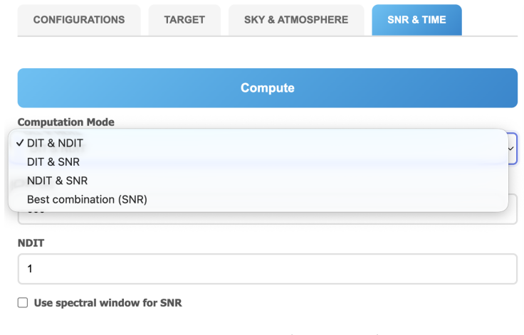
- The exposure-time inversion modes allow survey planners to convert a target SNR directly into a DIT/NDIT schedule, which is exactly what is needed for designing an observational campaign.
Where Pith is reading between the lines
- Editorial inference: because the throughput tables are the only unmeasured input, the same tool can be rerun with revised tables at every design iteration, turning the ETC into a living survey forecast.
- Editorial inference: the fibre-injection treatment could be sharpened by adding atmospheric dispersion and 3-D slit losses, which would most affect the blue end of each channel.
- Editorial inference: making the calculator public invites independent reproduction of the headline depths, which would test the design baseline without needing the telescope.
Editorial analysis
A structured set of objections, weighed in public.
Referee Report
Summary. The paper presents pyetc_wst, an exposure time calculator for the proposed Wide-field Spectroscopic Telescope, covering IFS, MOS-LR, and MOS-HR. It implements a source-to-detector photon budget (Eq. 1), static and SkyCalc sky backgrounds, PSF/fibre injection, a noise model (Eq. 2), four computation modes, and web/REST/CLI interfaces. Example outputs include SNR spectra, noise decomposition, and limiting magnitudes: IFS surface brightness μ_r ≈ 25.4 AB arcsec^-2 and MOS-LR point-source limits r ≈ 22–23.4 AB for 1 h dark-sky observations.
Significance. The main value of this work is a public, modular ETC implementation built on standard photon-budget and variance equations, with useful features such as SkyCalc integration, a rich SED/template library, flexible computation modes, and noise decomposition. These are concrete strengths that make the tool immediately usable for WST survey planning. However, the quantitative performance predictions are not independent measurements: they scale linearly with preliminary system-engineering throughput tables that are explicitly subject to revision. The paper's claim that the throughput model and performance numbers are 'verified against first-principles expectations' goes beyond what is actually shown and should be tempered or supported by a sensitivity analysis.
major comments (2)
- [§5.3, §2.1] The claim that GLAO improves the IFS surface-brightness limit by reducing the sky background per spaxel is physically incorrect for a fixed 0.25″ spaxel. For a uniform extended source, both source and sky counts per spaxel are independent of PSF. If instead the extraction aperture is matched to the PSF, a smaller PSF reduces the aperture area and thus the SNR per resolution element. Fig. 10 and the headline μ_r ≈ 25.4 AB arcsec^-2 rest on this step. Please specify the exact spatial binning/resolution element and provide a derivation; as written, the GLAO-specific SB limiting magnitudes are unsupported.
- [§5.1, Fig. 8, §6] All limiting magnitudes and SNR curves scale linearly with the preliminary throughput tables T_ins(λ) in Eq. (1), which are unmeasured engineering estimates ('expected to reach' 79.8%/91.3% telescope throughput, assumed detector RON/dark) with no quoted uncertainty. The paper itself warns in §5.1 that 'all performance numbers reported in this paper should be interpreted accordingly,' yet §6 states the throughput model has been 'verified against first-principles expectations' and presents the limits as confirming WST performance. No verification or sensitivity analysis is shown. Please add an uncertainty propagation or sensitivity study for the headline numbers, or explicitly reframe the conclusions as provisional engineering estimates.
minor comments (5)
- [Throughout] The package name is typeset inconsistently as 'pyetc wst' in the text and 'pyetc_wst' in code/URLs; unify the notation.
- [Fig. 9 caption] The caption says 'rebinned by 5 Å for display' while the text describes SNR per spectral pixel; clarify whether the values are per native pixel or per rebinned bin.
- [§5.3] The definition 'per resolution element of 1.4 Å co-added over 3 spectral pixels' specifies only the spectral bin; the spatial element used for the IFS surface-brightness limit should be stated explicitly (e.g., 1 spaxel, N×N bin, or PSF area).
- [References] References [5], [6], and [7] cite 'Proc. SPIE This conference' with paper numbers but no page/article details; if available, add full bibliographic information or a DOI.
- [Table 1] The MOS-HR channels are named Blue, Green, Yellow, Red, which may be confused with the MOS-LR channels of the same names in Fig. 8. Consider adding the central wavelengths or a prefix (e.g., HR-Blue) to the channel labels.
Circularity Check
No circularity: the ETC results are conditional photon-budget calculations from explicitly preliminary instrument-throughput inputs.
full rationale
The derivation chain is a standard ETC photon budget: Eq. (1) computes detected signal as the product of source flux, telescope area, atmospheric transmission, instrument throughput, fibre fraction, and exposure time; Eq. (2) forms the noise variance and SNR; the limiting magnitudes in §5.3 are obtained by inverting SNR = 3. The instrument throughput T_ins is an input (Fig. 8), explicitly described as 'a preliminary throughput model delivered by the WST system engineering team' that 'will be updated as the design matures' (§5.1). Nothing in the paper defines T_ins in terms of the predicted SNR or limiting magnitudes, and no parameter is fitted to the output curves; the reported numbers are conditional on the stated engineering baseline. The §6 sentence claiming the model has been 'verified against first-principles expectations' is unsupported by the text, but that is a validation/evidence gap, not a circular reduction: nothing shows the prediction being used to construct its own input. The self-references to WST design papers (refs [4]–[7]) provide design parameters such as coating expectations, not a uniqueness theorem or an ansatz, and the central calculation does not collapse into those citations. An ETC can, in principle, be checked against independent end-to-end simulations or future as-built measurements, so the central derivation retains independent content. The appropriate concern—unquantified throughput uncertainty affecting all limiting magnitudes—is a correctness risk, not circularity.
Axiom & Free-Parameter Ledger
free parameters (6)
- Instrument throughput tables T_ins(λ) per channel =
IFS blue ~34% peak, IFS red ~39% peak, MOS-LR 24–34%, MOS-HR 13–19% (Fig. 8)
- Telescope throughput 79.8% (IFS) / 91.3% (MOS) =
79.8% / 91.3% (§2.1)
- Detector RON and dark current per channel =
RON 1.0–1.4 e^-, dark 1–2 e^-/hr (Table 1)
- Moffat PSF β = 2.8 =
β = 2.8 (§3.2)
- GLAO image quality 0.5″ FWHM at 650 nm, 40% probability =
0.5″ at 650 nm, 40% probability, 85% sky coverage (§2.1)
- Static-mode sky brightness levels (dark/grey/bright) =
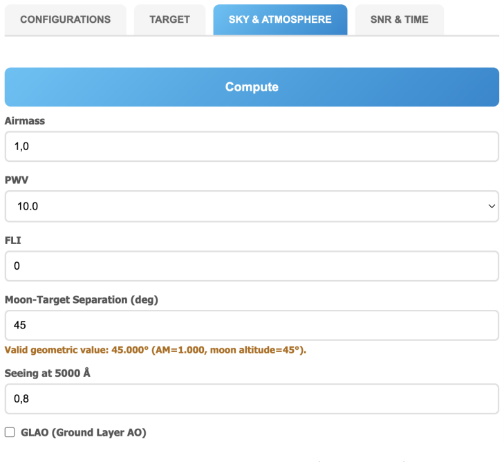
FLI = 0, 0.5, 1.0 (§3.3)
axioms (5)
- standard math Photon budget: detected electrons = F_λ × (λ/hc) × A_tel × τ_atm × T_ins × f_fib × t_exp (Eq. 1)
- standard math Noise variance = N_DIT × [S_src + S_sky + N_pix(d t_DIT + σ_RON²)] with Poisson source/sky and Gaussian RON (Eq. 2)
- domain assumption ESO SkyCalc emission/transmission spectra are representative of the WST site observing conditions
- ad hoc to paper The system-engineering throughput tables T_ins(λ) describe the as-built instrument
- domain assumption Moffat profile with β = 2.8 models on-sky PSF including seeing wings
Cite this review
Pith. "Pith review of WST instrument Exposure Time Calculator: full simulation of multi-mode spectrograph performance from source to detector." pith.science (2026). https://pith.science/paper/5GUYVUEG
@misc{pith2026260800193,
  author       = {Pith},
  title        = {Pith review of: WST instrument Exposure Time Calculator: full simulation of multi-mode spectrograph performance from source to detector},
  year         = {2026},
  howpublished = {\url{https://pith.science/paper/5GUYVUEG}},
  note         = {Machine review of arXiv:2608.00193}
}
read the original abstract
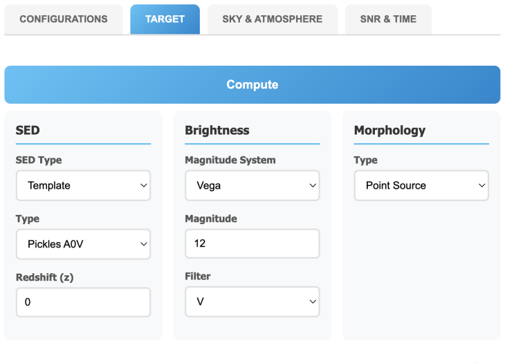
We present a comprehensive Exposure Time Calculator (ETC) developed for the Wide-field Spectroscopic Telescope (WST) concept. The WST, currently in its conceptual phase, is designed as a next-generation large spectroscopic survey facility featuring three complementary observing modes: an Integral Field Spectrograph (IFS) covering 370-930 nm at R of about 4800; a high-resolution Multi-Object Spectrograph (MOS-HR) with four bands at R of about 40000; and a low-resolution Multi-Object Spectrograph (MOS-LR) with four channels at R of about 3800-4900. The ETC simulates the complete photon-propagation path from astronomical source to detector, incorporating wavelength-dependent system throughput (telescope transmission, instrumental optics, detector quantum efficiency), accurate sky background via ESO SkyCalc integration, and a comprehensive noise treatment (photon noise, sky background, read-out noise, dark current). The computational core is implemented as the "pyetc_wst" Python library built on the MPDAF framework, supporting multiple target spectral energy distributions (stellar templates, blackbody, power-law, emission lines, and user-uploaded spectra with arbitrary redshift) and spatial morphologies (point sources and Sersic extended profiles). Four operational modes enable flexible exposure-time optimization. Full spectral outputs include wavelength-dependent signal-to-noise ratio (SNR), source and sky photon counts, noise decomposition by component, and simulated extracted spectra. An interactive web interface, together with a REST API and a command-line tool, complete the user experience and enable batch survey-design workflows.
Figures




Reference graph
Works this paper leans on
-
[1]
An atmospheric radiation model for Cerro Paranal,
Noll, S., Kausch, W., Barden, M., Jones, A. M., Szyszka, C., Kimeswenger, S., and Vinther, J., “An atmospheric radiation model for Cerro Paranal,”Astron. Astrophys.543, A92 (2012)
2012
-
[2]
An advanced scattered moonlight model for Cerro Paranal,
Jones, A., Noll, S., Kausch, W., Szyszka, C., and Kimeswenger, S., “An advanced scattered moonlight model for Cerro Paranal,”Astron. Astrophys.560, A91 (2013)
2013
-
[3]
MPDAF – A Python package for the analysis of VLT/MUSE data,
Bacon, R. et al., “MPDAF – A Python package for the analysis of VLT/MUSE data,” in [Astronomical Data Analysis Software and Systems XXV],ASP Conf. Ser.507, 427 (2016)
2016
-
[4]
The Wide-field Spectroscopic Telescope (WST) science white paper,
Mainieri, V., de Jong, R. S., Bacon, R., and WST Collaboration, “The Wide-field Spectroscopic Telescope (WST) science white paper,” in [Proc. SPIE],Proc. SPIE13094(2024). arXiv:2403.05398
Pith/arXiv arXiv 2024
-
[5]
Progress of the design of the 12-m optical, Wide-Field Spectroscopic Telescope (WST),
Dierickx, P. and WST Collaboration, “Progress of the design of the 12-m optical, Wide-Field Spectroscopic Telescope (WST),” in [Proc. SPIE],Proc. SPIEThis conference(2026). Paper No: 14147-196
2026
-
[6]
WST - Widefield Spectroscopic Telescope: the next leap in wide-field spectroscopy. ,
Bacon, R. and WST Collaboration, “WST - Widefield Spectroscopic Telescope: the next leap in wide-field spectroscopy. ,” in [Proc. SPIE],Proc. SPIEThis conference(2026). Paper No: 14147-18
2026
-
[7]
Widefield Spectroscopic Telescope (WST): coating strategy to achieve high optical throughput. ,
Sassolas, B. and WST Collaboration, “Widefield Spectroscopic Telescope (WST): coating strategy to achieve high optical throughput. ,” in [Proc. SPIE],Proc. SPIEThis conference(2026). Paper No: 14147-100
2026
-
[8]
A theoretical investigation of focal stellar images in the photographic emulsion and application to photographic photometry,
Moffat, A. F. J., “A theoretical investigation of focal stellar images in the photographic emulsion and application to photographic photometry,”Astron. Astrophys.3, 455–461 (1969)
1969
-
[9]
skycalc cli: ESO SkyCalc Command-Line Interface
ESO, “skycalc cli: ESO SkyCalc Command-Line Interface.”https://pypi.org/project/skycalc-cli/ (2023)
2023
-
[10]
A grid of MARCS model atmospheres for late-type stars,
Gustafsson, B., Edvardsson, B., Eriksson, K., Jørgensen, U. G., Nordlund, ˚A., and Plez, B., “A grid of MARCS model atmospheres for late-type stars,”Astron. Astrophys.486, 951–970 (2008)
2008
-
[11]
A stellar spectral flux library: 1150–25000 ˚A,
Pickles, A. J., “A stellar spectral flux library: 1150–25000 ˚A,”Publ. Astron. Soc. Pacific110, 863–878 (1998)
1998
-
[12]
ATLAS9 Stellar Atmosphere Programs and 2 km/s grid
Kurucz, R. L., “ATLAS9 Stellar Atmosphere Programs and 2 km/s grid.” CD-ROM No. 13, Smithsonian Astrophysical Observatory (1993)
1993
-
[13]
A new extensive library of PHOENIX stellar atmospheres and synthetic spectra,
Husser, T.-O., Wende-von Berg, S., Dreizler, S., Homeier, D., Reiners, A., Barman, T., and Hauschildt, P. H., “A new extensive library of PHOENIX stellar atmospheres and synthetic spectra,”A&A553, A6 (2013)
2013
-
[14]
Tem- plate ultraviolet to near-infrared spectra of star-forming galaxies and their application to K-corrections,
Kinney, A. L., Calzetti, D., Bohlin, R. C., McQuade, K., Storchi-Bergmann, T., and Schmitt, H. R., “Tem- plate ultraviolet to near-infrared spectra of star-forming galaxies and their application to K-corrections,” Astrophys. J.467, 38–60 (1996)
1996
-
[15]
SWIRE template library
Polletta, M., “SWIRE template library.”https://www.iasf-milano.inaf.it/ ~polletta/templates/ swire_templates.html(2007). Accessed: 2026
2007
-
[16]
pyetc wst: WST Exposure Time Calculator
Ferro, M. et al., “pyetc wst: WST Exposure Time Calculator.”https://github.com/ferromatteo/ pyetc_wst(2026)
2026
-
[17]
Array programming with NumPy,
Harris, C. R. et al., “Array programming with NumPy,”Nature585, 357–362 (2020)
2020
-
[18]
SciPy 1.0: Fundamental algorithms for scientific computing in Python,
Virtanen, P. et al., “SciPy 1.0: Fundamental algorithms for scientific computing in Python,”Nature Meth- ods17, 261–272 (2020)
2020
-
[19]
The Astropy Project: Sustaining and growing a community-developed open- source project and status of the v2.0 core package,
Astropy Collaboration et al., “The Astropy Project: Sustaining and growing a community-developed open- source project and status of the v2.0 core package,”Astron. J.156, 123 (2018)
2018
This paper was first reviewed by deepseek-v4-flash on August 4, 2026.
discussion (0)
Sign in with ORCID, Apple, or X to comment. Anyone can read and Pith papers without signing in.