REVIEW 3 major objections 5 minor 87 references
Duck hunting with quantum mechanics
T0 review · 3 major / 5 minor · reviewed 2026-08-05 · deepseek-v4-flash
Pith's one-line read Canard trajectories in a slow-fast system are shown to be quantum instantons: the duck window width is exp(-S/2ω).
desk verdict A plausible and genuinely synthetic paper whose central exact quantization condition has an internal sign discrepancy that must be fixed before the results can be relied on. read the letter →
The pith
A machine-rendered reading of the paper's core claim, the machinery that carries it, and where it could break.
The reading
What carries the argument
The workhorse is the chain Möbius system ↔ Riccati ↔ Schrödinger. On the torus with first-mode-only Fourier dependence, the first-return map is a Möbius transformation; converting to the Riccati variable Φ makes the critical curve an elliptic curve with two homology cycles, and the Riccati equation transforms to a zero-energy Schrödinger equation. The α-cycle integral fixes band centers via a quantization condition, the β-cycle integral is the instanton action that sets the exponentially small band and canard width, and the exact DDP quantization condition (eq. 40) locates band-gap edges from two phases and a barrier exponent.
What would settle it
Numerically compute, for fixed small ω (e.g. 0.05) and fixed A, the set of B values for which generic initial conditions produce a canard segment on the unstable branch over O(1) slow time, and compare the measured width to exp(-S_inst/(2ω)) from the β-cycle integral; in parallel, evaluate the monodromy matrix trace at the predicted band edges from eq. (40) and check |tr M| = 2 to within numerical precision.
Extended reading notes
Core claim
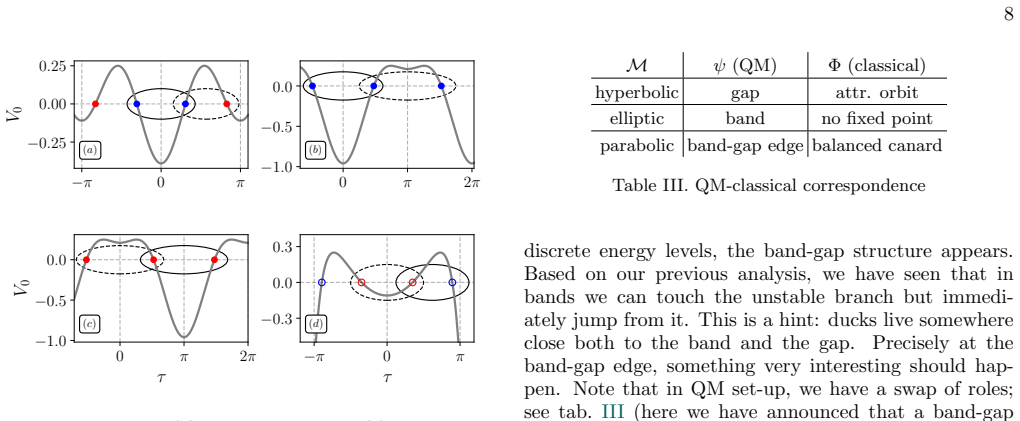
The paper's core discovery is an exact bridge between canard existence and instanton-controlled band-gap edges. For systems whose fast variable satisfies a Möbius-type first-return map, the Riccati equation can be linearized into a zero-energy Schrödinger equation, so canard questions become band-gap questions. The paper argues that canards occur precisely at the parabolic monodromy points |tr M|=2, i.e., at band-gap edges, and that the width of the parameter layer where generic initial conditions produce canards is exp(-S_inst/(2ω)), where S_inst is the integral of sqrt(V0) over the β-cycle of the underlying elliptic curve. For the overdamped Josephson junction, the canard window is the exp
Load-bearing premise
The load-bearing premise is that the canard window exactly coincides with the exponentially thin layer around the parabolic monodromy points, and that the phase relation θ2 = θ1 - Im Iβ + πB/ω in eq. (40) is exact; if this phase relation fails, the predicted band edges and canard windows shift.
Editorial extensions
If this is right
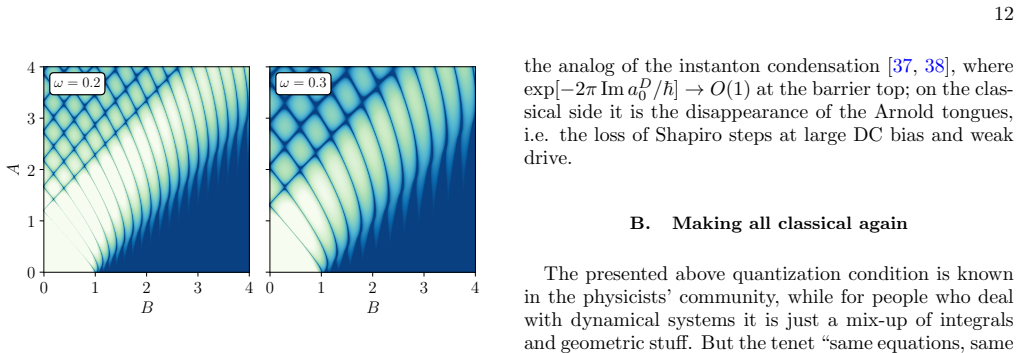
- In the overdamped Josephson junction, the Shapiro-step risers are exponentially narrow (width exp(-S_inst/2ω)) and are populated by canard trajectories; the DC voltage changes by ħω/2e over an exponentially small bias interval.
- The catalog of canards (maximal, headless, balanced, duck-that-never-jumps) is organized by the ratio of the budget banked on the unstable branch, S_+/S_inst, and the winding number, as summarized in the balance law and catalog table.
- The double-resonance condition B = lω that creates the constrictions is protected by an exact residue relation and receives no ω-corrections, producing a minigap structure in the 2FP regime.
- Because the formal expansion is Gevrey-1 and only even ω-powers contribute to cycle integrals, the exact-WKB procedure automatically incorporates higher-order ω-corrections, extending the leading-order picture beyond the exponentially thin band.
- At the boundary |A|=|B|-1 with |B|>1, the β-cycle degenerates, S_inst→0, and the exponential width saturates to O(1), signaling the loss of Shapiro steps and the analog of instanton condensation.
Reading between the lines
- The same dictionary should apply to any Möbius-type torus system whose associated potential V0 has the same well-barrier structure; the window-width formula for canard observability is testable without invoking a quantum interpretation.
- The sign of the πB/ω phase in eq. (40) versus Appendix E is not settled in the paper; a high-precision numerical monodromy test at a predicted band edge would reveal which sign is correct and shift the location of the ducks accordingly.
- The exponential sensitivity of canard observability implies a precision cost of roughly 0.434 S/ω decimal digits to resolve a duck segment, which sets a practical bound for neuromorphic or superconducting device applications.
- The noise-suppression results cited for canards could be recast as a large-deviation principle for the zero-energy Schrödinger problem, potentially giving an instanton-based estimate of how noise shrinks the canard window.
Editorial analysis
A structured set of objections, weighed in public.
Referee Report
Summary. The paper proposes a dictionary between canard trajectories in slow-fast systems on a torus and non-perturbative (instanton) effects in exact WKB theory, using the overdamped resistively shunted Josephson junction as the concrete example. After rewriting the RSJ equation as a Riccati equation and then as a zero-energy Schrödinger equation, the author expresses the relevant monodromy data in terms of α- and β-cycle integrals on an associated elliptic curve, writes an exact DDP-type quantization condition, and identifies band-gap edges (parabolic monodromy) with balanced canards. The central quantitative claims are that the canard window in parameter space has width exp(−S_inst/2ω), where S_inst is the β-cycle instanton action, and that this window is the exponentially narrow riser between consecutive Shapiro steps. The paper contains analytic computations of the cycle integrals, several regime decompositions, a catalog of canard types, and numerical trajectories at parameters selected by the quantization conditions.
Significance. If the central identification is correct, the paper provides a striking and genuinely parameter-free bridge between two previously separate bodies of results: classical canard theory and exact WKB/instanton analysis. The concrete payoff is a falsifiable prediction for the RSJ model: the location and exponential width of canard windows coincide with the gaps between Shapiro steps, with S_inst computed analytically from the model. Strengths include the absence of fitted parameters in the main derivation, the explicit elliptic-integral evaluation of the cycle integrals, and numerical canard trajectories generated at parameters chosen a priori from the quantization condition. These features make the paper potentially important for both the dynamical-systems and semiclassical/instanton communities. However, the central claim is currently weakened by an internal sign inconsistency in the phase relation defining the exact quantization condition, and by the fact that the key identification between canard existence and parabolic monodromy is asserted rather than derived.
major comments (3)
- [§V.A, Eq. (40) vs Appendix E] The exact quantization condition defines θ2 = θ1 − Im Iβ + πB/ω, while Appendix E derives first θ2 = θ1 − πB/ω and then states that “we have to add −Im Iβ contribution,” yielding θ2 = θ1 − Im Iβ − πB/ω. These differ by 2πB/ω, which is not exponentially small: because θ1 ∼ Iα/(2ω), the sign flip changes the arguments of cos(θ1+θ2) and cos θ1 cos θ2 by an O(1) amount in B at fixed A and ω. Since the band-gap edges are located by |tr M| = 2, this O(1) shift moves the predicted canard window. The main text and Appendix E cannot both be correct, and no numerical check in the paper resolves the discrepancy. This must be fixed before the central claim is established.
- [§IV.A and §IV.E] The claim that the forward-observable canard layer has width exp(−S_inst/2ω) is asserted from a balance-law heuristic. Eq. (37) gives S+ = (S_inst + ω ln Λ)/2, and at the parabolic edge Λ=1 one obtains S+ = S_inst/2, which justifies the statement that the balanced canard banks half the instanton action. It does not, by itself, imply that in parameter space the set of parameters for which generic initial conditions display canards has width exp(−S_inst/2ω). A derivation from the monodromy trace near the parabolic point (or an explicit numerical verification of this width) is needed. As it stands, the paper’s headline formula “log of canard window = scaled instanton action” is supported only at the level of scaling heuristics.
- [§IV.E, Table III] The identification of canard solutions with parabolic monodromy points |tr M| = 2 is announced rather than proved. Table III states simply that parabolic monodromy corresponds to a “balanced canard,” but no argument is given that at (or exponentially near) the band-gap edge the stable and unstable periodic orbits merge and the resulting trajectory rides the unstable branch for O(1) slow time. This is a load-bearing point of the paper: the entire dictionary and the numerical selection of parameters in Figs. 9–10 depend on it. The author should either provide a proof using the contraction/expansion estimates of §IV.B or cite a theorem that establishes this correspondence for Möbius systems.
minor comments (5)
- [§IV (intro)] “hunting riffle” should presumably be “hunting rifle”.
- [§V.A] The quantization condition (40) is called “full and exact,” but all numerical band-gap structures shown are evaluated with leading-order α- and β-cycle integrals. The paper should state explicitly whether the plotted curves include ω-corrections from p(τ,ω), and if not, what accuracy the leading-order approximation is expected to have.
- [Appendix D] The appendix derives explicit formulas for the α- and β-cycle integrals only in the 2FP regime and states that other regimes are obtained by T-duality/Dehn-twist transformations, but it does not give the resulting final expressions. A reader cannot verify the branch choices or the signs of the pole contributions without repeating the computation. Adding the explicit SFP and NFP formulas would increase reproducibility.
- [§II.D, Eq. (19)] The exact identity ω(N> − N<) = πB is stated to hold for |A|>|B|+1. The derivation via contour deformation is sketched in one sentence; a few more details (or a reference to the appendix where the residue is computed) would help.
- [References] The paper relies on two companion preprints by the author, [55] and [68], for the rotation number quantization and for the rigorous validity of the harmonic quantization condition. If these are not yet published, the dependence should be flagged in the text.
Circularity Check
No significant circularity: the central derivation is self-contained and prediction-checked. A sign discrepancy between Eq. (40) and Appendix E is a correctness risk, not a circular reduction.
full rationale
The paper's central chain is: RSJ model -> Riccati -> Schrödinger -> elliptic curve α/β cycles -> DDP quantization condition -> numerical canard generation. The key quantities S_inst, I_α, and I_β are computed analytically from the model, not fitted to canard data. Canard trajectories in Figs. 8–10 are then generated at parameters selected via the quantization condition, which is a genuine prediction-check rather than a re-use of fitted inputs. The only self-citation is [55] (Alexandrov, Glutsyuk, Gorsky), cited for the remark that rotation-number quantization is "true quantum-mechanical quantization"; this is not load-bearing for the canard-window derivation, and the central result is independently derived from the DDP formula [69,70] and elliptic integrals. The identification "parabolic monodromy = balanced canard" (Table III, §IV.E) is asserted and then supported by the Floquet balance law S_+ = (S_inst + ω ln Λ)/2, with numerical confirmation in Fig. 9; it is not a definitional reduction. One real problem exists but is not circularity: Eq. (40) sets θ2 = θ1 − Im Iβ + πB/ω, while Appendix E derives θ2 = θ1 − πB/ω and then adds −Im Iβ, giving θ2 = θ1 − Im Iβ − πB/ω. This 2πB/ω sign discrepancy would shift the predicted band-edge locations, so the exact boundaries of the canard window are not yet settled. However, this is an internal inconsistency/correctness issue, not a case of the output being equivalent to the input by construction.
Assumptions & free parameters
free parameters (1)
- ζ (canard fraction) =
chosen by hand, 0<ζ<1 (examples not specified)
assumptions (5)
- domain assumption Möbius system restriction: F(τ,φ) has only first Fourier modes in φ, making the first recurrence map a Möbius transformation.
- standard math Riccati variable transformation Φ = -ψ'/(f+ψ) followed by gauge ψ → sqrt(f+) ψ maps the ODE to a linear Schrödinger equation.
- standard math Fenichel theory and exponentially small splitting of slow manifolds: canards arise when the splitting vanishes.
- ad hoc to paper Exact DDP quantization condition (40) with θ2 = θ1 - Im Iβ + πB/ω is exact and its continuation across regimes is valid.
- ad hoc to paper Canard locus coincides with parabolic monodromy points |tr M|=2 (band-gap edges), and the forward-observable canard layer has width exp(-S_inst/2ω).
Cite this review
Pith. "Pith review of Duck hunting with quantum mechanics." pith.science (2026). https://pith.science/paper/W6SBJNCR
@misc{pith2026260800579,
  author       = {Pith},
  title        = {Pith review of: Duck hunting with quantum mechanics},
  year         = {2026},
  howpublished = {\url{https://pith.science/paper/W6SBJNCR}},
  note         = {Machine review of arXiv:2608.00579}
}
read the original abstract
We bridge two sides of singular perturbation theory: the classical theory of slow-fast systems and the semi-classical approach to quantum mechanical systems. For a specific but physically important class of dynamical systems, we show that purely classical and exotic objects, so-called canard solutions, are shadows of instantons in the corresponding quantum system. We demonstrate that canard solutions exist in a domain of parameter space whose boundaries are determined by an instanton action. We illustrate our statements analytically for the relevant example, the overdamped Josephson junction, and confirm them numerically. For the Josephson junction, the canard window is the exponentially narrow gap between consecutive Shapiro steps.
Figures


Figures from the paper (8 more)





Reference graph
Works this paper leans on
-
[1]
The main difference from the usual case is that our form has poles atu=±i
(u2 −u 2∞) (1 +u 2)2 du,(B4) whereC= p 1−(A−B) 2. The main difference from the usual case is that our form has poles atu=±i. Residues at these poles are Res u=±i Ω =±B.(B5) Finally, let us discuss the elliptic curve that appears in the QM-based approach. We have p2 0 =− (1−B−Acosτ)(1 +B+Acosτ) 4 ,(B6) wherep 0 is a classical momentum. It is easy to see th...
-
[2]
Notice that S- duality holds:k 2 β +k 2 α = 1, wherek 2 β is eq
sin2 ϕ,(D10) which gives Iβ = C(u 2 ∞ −u 2 0)2 u∞(1 +u 2∞)2 Z π/2 0 dϕsin 2 ϕcos 2 ϕ (1−nsin 2 ϕ)2 p 1−k 2 sin2 ϕ , (D11) withkandnare k2 = 4A (A+ 1) 2 −B 2 , n= 2 A−B+ 1 .(D12) Again, the last integral can be decomposed into the com- bination of complete elliptic integrals. Notice that S- duality holds:k 2 β +k 2 α = 1, wherek 2 β is eq. (D12) andk α is ...
-
[3]
Kawai and Y
T. Kawai and Y. Takei,Algebraic Analysis of Singu- lar Perturbation Theory, Translations of Mathematical Monographs, Vol. 227 (American Mathematical Society, Providence, RI, 2005)
2005
-
[4]
S. R. S. Varadhan, Communications on Pure and Applied Mathematics19, 261 (1966)
1966
-
[5]
Touchette, Physics Reports478, 1 (2009)
H. Touchette, Physics Reports478, 1 (2009)
2009
-
[6]
Dembo and O
A. Dembo and O. Zeitouni,Large Deviations Techniques and Applications, 2nd ed., Stochastic Modelling and Ap- plied Probability, Vol. 38 (Springer, Berlin, Heidelberg, 2010)
2010
-
[7]
M. I. Freidlin and A. D. Wentzell,Random Perturbations of Dynamical Systems, 3rd ed., Grundlehren der math- ematischen Wissenschaften, Vol. 260 (Springer, Berlin, Heidelberg, 2012)
2012
-
[8]
Prandtl, inVerhandlungen des III
L. Prandtl, inVerhandlungen des III. Internationalen Mathematiker-Kongresses, Heidelberg 1904(Teubner, Leipzig, 1905) pp. 484–491
work page 1904
Show all 87 references
-
[9]
Schlichting and K
H. Schlichting and K. Gersten,Boundary-Layer Theory, 9th ed. (Springer, Berlin, Heidelberg, 2017)
2017
-
[10]
A. N. Tikhonov, Matematicheskii Sbornik31(73), 575 (1952)
1952
-
[11]
Fenichel, Journal of Differential Equations31, 53 (1979)
N. Fenichel, Journal of Differential Equations31, 53 (1979)
1979
-
[12]
C. K. R. T. Jones, inDynamical Systems (Montecatini Terme, 1994), Lecture Notes in Mathematics, Vol. 1609 (Springer, Berlin, Heidelberg, 1995) pp. 44–118
1994
-
[13]
Kuehn,Multiple Time Scale Dynamics, Applied Mathematical Sciences, Vol
C. Kuehn,Multiple Time Scale Dynamics, Applied Mathematical Sciences, Vol. 191 (Springer, Cham, 2015)
2015
-
[14]
L.-Y. Chen, N. Goldenfeld, and Y. Oono, Physical Re- view Letters73, 1311 (1994)
1994
-
[15]
L.-Y. Chen, N. Goldenfeld, and Y. Oono, Physical Re- view E54, 376 (1996)
1996
-
[16]
Beno ˆ ıt, J.-L
´E. Beno ˆ ıt, J.-L. Callot, F. Diener, and M. Diener, Col- lectanea Mathematica31–32, 37 (1981)
1981
-
[17]
Beno ˆ ıt, Ast´ erisque109–110, 159 (1983)
´E. Beno ˆ ıt, Ast´ erisque109–110, 159 (1983)
1983
-
[18]
Dumortier and R
F. Dumortier and R. Roussarie, Memoirs of the American Mathematical Society121, 10.1090/memo/0577 (1996)
1996 doi
-
[19]
Desroches and M
M. Desroches and M. R. Jeffrey, Proceedings of the Royal Society A: Mathematical, Physical and Engineering Sci- ences467, 2404 (2011)
2011
-
[20]
Moehlis, Journal of Mathematical Biology52, 141 (2006)
J. Moehlis, Journal of Mathematical Biology52, 141 (2006)
2006
-
[21]
Brøns and K
M. Brøns and K. Bar-Eli, The Journal of Physical Chem- istry95, 8706 (1991)
1991
-
[22]
Harvey, V
E. Harvey, V. Kirk, M. Wechselberger, and J. Sneyd, Journal of Nonlinear Science21, 639 (2011)
2011
-
[23]
H. G. Rotstein, M. Wechselberger, and N. Kopell, SIAM Journal on Applied Dynamical Systems7, 1582 (2008)
2008
-
[24]
Desroches, J
M. Desroches, J. Guckenheimer, C. Kuehn, B. Krauskopf, H. M. Osinga, and M. Wechselberger, SIAM Review54, 211 (2012)
2012
-
[25]
F. Zhan, S. Liu, X. Zhang, J. Wang, and B. Lu, Nonlinear Dynamics94, 807 (2018)
2018
-
[26]
Liu and S
Y. Liu and S. Liu, Nonlinear Dynamics101, 531 (2020)
2020
-
[27]
Desroches, T
M. Desroches, T. J. Kaper, and M. Krupa, Chaos23, 046106 (2013)
2013
-
[28]
T. Vo, R. Bertram, and M. Wechselberger, SIAM Journal on Applied Dynamical Systems12, 789 (2013)
2013
-
[29]
De Maesschalck, F
P. De Maesschalck, F. Dumortier, and R. H. Roussarie, Canard cycles: from birth to transition, Vol. 73 (Springer, 2021)
2021
-
[30]
Benoit, A
E. Benoit, A. El Hamidi, and A. Fruchard, Electronic Journal of Differential Equations2002, 1 (2002)
2002
-
[31]
Callot, Math´ ematiques finitaires et analyse non standard , 105 (1985)
J.-L. Callot, Math´ ematiques finitaires et analyse non standard , 105 (1985)
1985
-
[32]
Callot, Annales scientifiques de l’ ´Ecole Normale Sup´ erieure26, 149 (1993), s´ erie 4
J.-L. Callot, Annales scientifiques de l’ ´Ecole Normale Sup´ erieure26, 149 (1993), s´ erie 4
1993
-
[33]
J.-L. Callot,Bifurcations du portrait de phase pour des ´ equations diff´ erentielles lin´ eaires du second ordre ayant pour type l’´ equation d’Hermite, Th` ese, Universit´ e Louis Pasteur, Strasbourg, Strasbourg (1981), institut de Recherche Math´ ematique Avanc´ ee (IRMA); ...
1981
-
[34]
Guckenheimer and Y
J. Guckenheimer and Y. Ilyashenko, Moscow Mathemat- 19 ical Journal1, 27 (2001)
2001
-
[35]
Shchurov, Transactions of the Moscow Mathematical Society71, 175 (2010)
I. Shchurov, Transactions of the Moscow Mathematical Society71, 175 (2010)
2010
-
[36]
Schurov and N
I. Schurov and N. Solodovnikov, Journal of Dynamical and Control Systems23, 481 (2017)
2017
-
[37]
Sueishi, S
N. Sueishi, S. Kamata, T. Misumi, and M. ¨Unsal, Journal of High Energy Physics2020, 114 (2020)
2020
-
[38]
Sueishi, S
N. Sueishi, S. Kamata, T. Misumi, and M. ¨Unsal, Journal of High Energy Physics2021, 96 (2021)
2021
-
[39]
G. V. Dunne and M. ¨Unsal, inResurgence, physics and numbers(Springer, 2017) pp. 249–298
2017
-
[40]
Ba¸ sar, G
G. Ba¸ sar, G. V. Dunne, and M. ¨Unsal, Journal of High Energy Physics2017, 087 (2017), arXiv:1701.06572 [hep- th]
2017 arXiv
-
[41]
Nikolaev, Nagoya Mathematical Journal250, 434 (2023), arXiv:2008.06492 [math.CA]
N. Nikolaev, Nagoya Mathematical Journal250, 434 (2023), arXiv:2008.06492 [math.CA]
2023 arXiv
-
[42]
Nikolaev, An exact perturbative existence and unique- ness theorem (2022), arXiv:2201.04526 [math.CA]
N. Nikolaev, An exact perturbative existence and unique- ness theorem (2022), arXiv:2201.04526 [math.CA]
2022 arXiv
-
[43]
Nikolaev, Communications in Mathematical Physics 400, 463 (2023), arXiv:2106.10248 [math.AP]
N. Nikolaev, Communications in Mathematical Physics 400, 463 (2023), arXiv:2106.10248 [math.AP]
2023 arXiv
-
[44]
Nikolaev, Geometry and resurgence of WKB solu- tions of Schr¨ odinger equations (2024), arXiv:2410.17224 [math.DG]
N. Nikolaev, Geometry and resurgence of WKB solu- tions of Schr¨ odinger equations (2024), arXiv:2410.17224 [math.DG]
2024 arXiv
-
[45]
Nikolaev, L’Enseignement Math´ ematique70, 251 (2024), arXiv:2112.08792 [math.CV]
N. Nikolaev, L’Enseignement Math´ ematique70, 251 (2024), arXiv:2112.08792 [math.CV]
2024 arXiv
-
[46]
K. U. Kristiansen and P. Szmolyan, Journal of Differen- tial Equations406, 202 (2024)
2024
-
[47]
K. U. Kristiansen and P. Szmolyan, Studies in Ap- plied Mathematics155, e70141 (2025), arXiv:2501.10707 [math-ph]
2025 arXiv
-
[48]
K. U. Kristiansen, A geometric approach to exponentially small splitting: The generic zero-hopf bifurcation of co- dimension two (2026), arXiv:2603.12103 [math.DS]
2026 arXiv
-
[49]
Dorigoni, Annals of Physics409, 167914 (2019)
D. Dorigoni, Annals of Physics409, 167914 (2019)
2019
-
[50]
Aniceto, G
I. Aniceto, G. Ba¸ sar, and R. Schiappa, Physics Reports 809, 1 (2019)
2019
-
[51]
´Ecalle, inBifurcations and periodic orbits of vector fields(Springer, 1993) pp
J. ´Ecalle, inBifurcations and periodic orbits of vector fields(Springer, 1993) pp. 75–184
1993
-
[52]
Eckhaus, inAsymptotic Analysis II, Lecture Notes in Mathematics, Vol
W. Eckhaus, inAsymptotic Analysis II, Lecture Notes in Mathematics, Vol. 985 (Springer, 1983) pp. 449–494
1983
-
[53]
Krupa and P
M. Krupa and P. Szmolyan, Journal of Differential Equa- tions174, 312 (2001)
2001
-
[54]
Krupa and P
M. Krupa and P. Szmolyan, SIAM Journal on Mathe- matical Analysis33, 286 (2001)
2001
-
[55]
Jard´ on-Kojakhmetov and C
H. Jard´ on-Kojakhmetov and C. Kuehn, inMexican Mathematicians in the World, Contemporary Mathemat- ics, Vol. 775, edited by F. Galaz-Garc ´ ıa, C. Gonz´ alez- Tokman, and J. C. Pardo Mill´ an (American Mathe- matical Society, Providence, RI, 2021) pp. 115–160, arXiv:1901.0140...
2021 arXiv
-
[56]
Buchstaber, O
V. Buchstaber, O. Karpov, and S. Tertychniy, Theoreti- cal and Mathematical Physics162, 211 (2010)
2010
-
[57]
Alexandrov, A
A. Alexandrov, A. Glutsyuk, and A. Gorsky, Journal of High Energy Physics2026, 101 (2026)
2026
-
[58]
K. K. Likharev,Dynamics of Josephson Junctions and Circuits(Gordon and Breach, New York, 1986)
1986
-
[59]
Barone and G
A. Barone and G. Patern` o,Physics and Applications of the Josephson Effect(Wiley, New York, 1982)
1982
-
[60]
Shapiro, Physical Review Letters11, 80 (1963)
S. Shapiro, Physical Review Letters11, 80 (1963)
1963
-
[61]
Panghotra, B
R. Panghotra, B. Raes, C. C. de Souza Silva, I. Cools, W. Keijers, J. E. Scheerder, V. V. Moshchalkov, and J. Van de Vondel, Communications Physics3, 53 (2020)
2020
-
[62]
Stolyarov, S
V. Stolyarov, S. Kozlov, D. Yakovlev, O. Skryabina, D. Lvov, A. Vasenko, J. Zhou, M. Y. Kupriyanov, A. Gol- ubov, C. Feuillet-Palma,et al., Communications Materi- als7, 91 (2026)
2026
-
[63]
Canalis-Durand, J.-P
M. Canalis-Durand, J.-P. Ramis, R. Sch¨ afke, and Y. Sibuya, J. Reine Angew. Math.518, 95 (2000)
2000
-
[64]
Beno ˆ ıt, A
´E. Beno ˆ ıt, A. Fruchard, R. Sch¨ afke, and G. Wallet, Ann. Fac. Sci. Toulouse Math. (6)7, 627 (1998)
1998
-
[65]
Fruchard and R
A. Fruchard and R. Sch¨ afke,Composite Asymptotic Expansions, Lecture Notes in Mathematics, Vol. 2066 (Springer, Berlin, Heidelberg, 2013) pp. x+161
-
[66]
Fruchard and R
A. Fruchard and R. Sch¨ afke, Discrete Contin. Dyn. Syst. Ser. S2, 931 (2009)
2009
-
[67]
Glutsyuk, V
A. Glutsyuk, V. Kleptsyn, D. Filimonov, and I. Schurov, Functional Analysis and Its Applications48, 272 (2014)
2014
-
[68]
Glutsyuk, Journal of Dynamical and Control Systems 25, 323 (2019)
A. Glutsyuk, Journal of Dynamical and Control Systems 25, 323 (2019)
2019
-
[69]
M. J. Renne and D. Polder, Revue de physique appliqu´ ee 9, 25 (1974)
1974
-
[70]
Glutsyuk, On phase-lock area parquet in a special slow-fast limit of model of josephson junction (2026), arXiv:2607.26158 [math.DS]
A. Glutsyuk, On phase-lock area parquet in a special slow-fast limit of model of josephson junction (2026), arXiv:2607.26158 [math.DS]
2026 arXiv
-
[71]
Dillinger, E
H. Dillinger, E. Delabaere, and F. Pham, Annales de l’Institut Fourier43, 163 (1993)
1993
-
[72]
Delabaere, H
E. Delabaere, H. Dillinger, and F. Pham, Journal of Mathematical Physics38, 6126 (1997)
1997
-
[73]
I. M. Gel’fand and L. A. Dikii, Russian Mathematical Surveys30, 77 (1975)
1975
-
[74]
K. U. Kristiansen, A geometric approach to exponentially small splitting: Zero-hopf bifurcations of arbitrary co- dimension (2026), arXiv:2603.12115 [math.DS]
2026
-
[75]
V. K. Mel’nikov, Transactions of the Moscow Mathemat- ical Society12, 1 (1963)
1963
-
[76]
Gelfreich, Physica D: Nonlinear Phenomena101, 227 (1997)
V. Gelfreich, Physica D: Nonlinear Phenomena101, 227 (1997)
1997
-
[77]
V. G. Gelfreich and V. F. Lazutkin, Russian Mathemat- ical Surveys56, 499 (2001)
2001
-
[78]
Guardia, C
M. Guardia, C. Oliv´ e, and T. M. Seara, Journal of Non- linear Science20, 595 (2010)
2010
-
[79]
D. V. Treschev, Chaos6, 6 (1996)
1996
-
[80]
D. V. Treschev, Regular and Chaotic Dynamics2, 9 (1997), in Russian
1997
-
[81]
D. V. Treschev, inProceedings of the International Congress of Mathematicians, Beijing 2002, Vol. 3 (2002) pp. 383–394, arXiv:math/0304459
2002 arXiv
-
[82]
A. I. Neishtadt, Differential Equations23, 1385 (1987), translated from Differentsial’nye Uravneniya23(1987), no. 12, 2060–2067
1987
-
[83]
A. I. Neishtadt, Differential Equations24, 171 (1988), translated from Differentsial’nye Uravneniya24(1988), no. 2, 226–233
1988
-
[84]
Berglund, B
N. Berglund, B. Gentz, and C. Kuehn, Journal of Differ- ential Equations252, 4786 (2012)
2012
-
[85]
R. B. Sowers, Journal of Theoretical Probability21, 824 (2008)
2008
-
[86]
Ginoux and J
J.-M. Ginoux and J. Llibre, Qualitative Theory of Dy- namical Systems15, 383 (2016)
2016
-
[87]
P. F. Byrd and M. D. Friedman,Handbook of El- liptic Integrals for Engineers and Scientists, 2nd ed., Die Grundlehren der mathematischen Wissenschaften, Vol. 67 (Springer-Verlag, Berlin, Heidelberg, New York, 1971)
1971
Reviewed August 5, 2026 · model on record in the stance chip above.
Discussion (0). Sign in to comment.