REVIEW 4 major objections 5 minor 50 references
Dependency Triad: A Metric to Quantify the Dependencies Between Attributes for Local Differential Privacy
T0 review · 4 major / 5 minor · reviewed 2026-08-05 · deepseek-v4-flash
Pith's one-line read The paper claims that three parameters—α, β, δ—suffice to summarize pairwise dependency information for local differential privacy, producing a constant-time conservative upper bound on correlation-induced leakage.
desk verdict The three-parameter compression is a real idea, but the shipped algorithm's core privacy guarantee is unproven because the LP-based beta is never shown to match the theorem's exact-calibration beta. read the letter →
The pith
A machine-rendered reading of the paper's core claim, the machinery that carries it, and where it could break.
The reading
What carries the argument
The carrying object is the ratio vector Q=G⊘G′, the element-wise division of the two conditional distributions. The proof first relaxes all feasible likelihood ratios to the extreme interval [e^{-γ}, e^α] and solves the resulting linear-fractional problem, obtaining a closed-form bound (Theorem IV.1) that depends only on the extremes; a sparsity correction δ is then introduced (Theorem IV.3). The calibrated lower endpoint e^{-β} replaces e^{-γ} by matching the estimate to the exact CPL* at a chosen budget ε0, and Theorem IV.4 shows the resulting estimate is an upper bound for all larger budgets. Uncertainty in the known distribution enters as an entry-wise matrix Δ that widens α, β, δ to the
What would settle it
Take a pair of conditional distributions and an uncertainty matrix Δ, solve the exact maximization of Σ_{i∈S}(G_i−G′_i) over all feasible S,G,G′ by enumeration, and compare it with φ returned by the relaxed LP in Algorithm 1 (line 18). If φ is smaller than the exact maximum, compute DT's CPL estimate for ε>ε0 and compare with CPL* obtained by exhaustive search over S; an estimate below CPL* disproves the upper-bound claim for the algorithm as delivered.
Extended reading notes
Core claim
Given two correlated attributes X_k and X̂ with conditional probability vectors G and G′, the exact correlation-induced privacy leakage CPL* is the optimum of a ratio of linear forms over all subsets of X̂'s alphabet. The paper's central discovery is that the part of that distribution needed to upper-bound CPL* survives in just three scalars: α, the log of the largest (uncertainty-corrected) likelihood ratio; δ, the mass sitting on entries whose conditional denominator can be zero; and β, a calibrated lower ratio level obtained by matching the closed-form estimate to the exact CPL* at one chosen privacy budget ε0. With (α,β,δ) in hand, CPL is given by a piecewise closed-form expression, and
Load-bearing premise
The upper-bound guarantee is proven for a β calibrated against the exact CPL* at ε0, but Algorithm 1 actually derives β from a relaxed linear program whose solution φ is asserted, not proven, to be an upper bound on the calibration statistic; if φ falls below the true maximum, the delivered estimate could understate the true leakage.
Editorial extensions
If this is right
- A one-time offline computation of (α,β,δ) costs O(a²b^3.5) and occupies O(1) space; after that, CPL at any privacy budget is a constant-time lookup, making iterative privacy-budget search practical for high-cardinality attributes.
- Pairwise DT estimates compose through the sequential-composition bound into a total-leakage estimate for multidimensional records, so the triad serves as the building block, not the endpoint.
- When several prior distributions are available, using the range or standard deviation as Δ yields uncertainty-aware per-attribute budgets that deliberately sit below the nominal optimum, hedging against demographic shifts.
- Across five real datasets, DT's normalized error against exact CPL* stays below 0.025 for ε∈[0.01,10] and below 0.003 for ε≤1, so the conservative guarantee is tight where LDP is typically deployed.
- In attribute-inference attack experiments at matched utility, DT achieves attack resistance comparable to simple budget splitting while consuming a smaller total privacy budget.
Reading between the lines
- If the compression is as general as claimed, the same ratio-extremes-plus-calibration scheme should extend to approximate (ε,δ)-LDP mechanisms by adding a second slack term for the δ-privacy parameter; the paper lists this as future work, and the existing proof structure suggests the natural form.
- Because β is calibrated at one anchor budget ε0, tightness is guaranteed to degrade as ε moves far above ε0; a testable extension is a piecewise triad with multiple anchor budgets, which would tighten the bound in low-privacy regimes without breaking the upper-bound property.
- The two-sided sparsity slacks (δ̃, δ̂) derived in the proof are collapsed into a single δ for simplicity; on sparse or asymmetric distributions, keeping them separate would likely tighten the estimate while preserving the bound.
- The empirical role split—β dominates leakage in the strong-privacy regime and α in the weak-privacy regime—suggests the triad could serve as an interpretable pairwise feature for selecting which attribute pairs to collect jointly or which are most exposed to attribute inference.
Editorial analysis
A structured set of objections, weighed in public.
Referee Report
Summary. The paper proposes the Dependency Triad (DT), a three-parameter summary (α, β, δ) of a pairwise conditional distribution, intended to quantify correlation-induced privacy leakage (CPL) under local differential privacy. The authors extend the CPL optimization of [14] to settings with distributional uncertainty, give Algorithm 1 for computing DT (using a relaxed linear program), and give Algorithm 2 for constant-time CPL estimation. The central claims are that CPL-relevant pairwise dependency information can be compressed into three parameters, that the resulting estimator is a conservative upper bound on the exact CPL under distributional uncertainty, and that it scales to high-cardinality and sparse distributions. Experiments on synthetic and five real datasets compare DT with HCC-2/LTM, demonstrate privacy-budget calibration, attribute-inference resistance, and utility gains over random sampling.
Significance. If the theoretical claims are made rigorous, this is a useful contribution: it addresses a real limitation of existing CPL algorithms, which require ground-truth distributions and repeated per-budget computation. The paper ships an artifact link, includes extensive experiments on real datasets, and the idea of an uncertainty-aware, low-dimensional summary of CPL is appealing. However, the central privacy guarantee currently rests on several unproved or under-specified analytic steps, most importantly the relationship between the relaxed LP in Algorithm 1 and the exact calibration theorem. The contribution is therefore promising but conditional.
major comments (4)
- [§V-B, Algorithm 1 lines 18–22 vs. Theorem IV.4] Theorem IV.4 proves the upper-bound property for a β calibrated using exact CPL* at ε0. In the deployment path, Algorithm 1 obtains β from φ produced by the relaxed LP at line 18 and the formula (16). The paper asserts that this LP is a polynomial-time upper bound to the exact MILP, but no proof is given that (i) the LP optimum is at least max_{S,G,G'} Σ_{i∈S}(G_i−G'_i) over the uncertainty set, and (ii) the map φ ↦ β, and then β ↦ CPL, is monotone nondecreasing. Without (i)–(ii), the delivered (α,β,δ) may understate CPL, violating the core 'never understate' guarantee. This needs an explicit lemma with proof.
- [§IV-B, Theorem IV.1 and Appendix C] The proof sketch asserts that the maximum CPL over all G,G' sharing ratio vector Q equals the maximum over two-point instances supported only on the extreme ratios e^α and e^{-γ}. Appendix C proves the value for a relaxed constraint set (27), but the reduction from the exact ratio-constrained set H to the extreme-ratio set ilde H is only asserted: intermediate ratios with positive mass cannot simply be set to zero without changing Q, and the argument appears to yield a supremum rather than an attained maximum. Since Theorem IV.4 inherits this result, the equality needs a rigorous proof or a relaxation argument that establishes the upper bound directly.
- [§IV-C, Theorem IV.8 and Appendix J, Corollary J.1] The uncertainty-aware claim relies on Corollary J.1, which states that taking componentwise maxima of two characterizations gives an upper bound, justified by an 'easy' monotonicity of CPL in α, β, and δ. No proof of this monotonicity is provided, and it is not immediate from Corollary IV.7, which only addresses γ. This monotonicity is load-bearing: it justifies using the upper-bound φ from the LP and the entry-wise uncertainty box Δ. A proof for each parameter is needed.
- [§V-B, Algorithm 1 line 18] The LP constraint contains the denominator M_i^+ + M_i^-. When M_i^+ = M_i^- = 0, the constraint is 0 ≤ z_i ≤ 0/0, which is undefined. This occurs when U_i = L'_i and U'_i = L_i, in particular for zero-probability symbols with zero uncertainty—exactly the sparse-distribution regime the paper claims to support. The pseudocode must define a convention (e.g., drop the constraint or set z_i = 0) and state it formally.
minor comments (5)
- [§V-B, Algorithm 1 line 16] The line 'δ←min(1,max(δ, δ))' appears to contain a typo or variable shadowing; the global δ and the loop-local δ are confused. Please rename and clarify.
- [Figure 3 caption] The caption says 'Figure 3a and Figure 3a'; the second reference should be Figure 3b.
- [§IV-B3, toy example] The toy example states α=1.50, γ=1.38, δ=0 for both scenarios; it would help to state explicitly that α and γ are computed for a fixed ordered pair (x,x') and how the orientation that maximizes leakage is selected.
- [Table IV] The 'Near monotone likelihood ratio' row reports mean CPL estimation error 7.9e−4 at ε=0.1 but 2.5e−1 at ε=1 with a large standard deviation; the text should comment on this non-monotonicity in ε, since DT is intended to be tight in high-privacy regimes.
- [Throughout] Several theorem references in the text (e.g., 'Theorem IV.8' in the proof of Theorem IV.8, 'Theorem F' in Appendix F) are inconsistent or refer to the appendix by its letter. Please normalize numbering.
Circularity Check
Partial circularity: default DT's beta is fitted to CPL* at the anchor epsilon0->0, so low-epsilon agreement is by construction; the upper-bound theorem supplies independent content.
-
fitted input called prediction
[Section IV-B4 (Theorem IV.4 and Corollary IV.5); Section VI-C; Definition V.1 Eq. (16)]
"We first calibrate β by equating the analytical CPL expression to the exact leakage CPL* at the calibration budget ε0 and solving for β. ... DT corresponds to the (α, β, δ) method calibrated at ε0 = 0."
Theorem IV.4 defines β by inverting the estimator expression so that the estimated CPL equals CPL* at ε0. In the default case ε0→0 (Corollary IV.5), β is set from φ = max_{S,G,G'} Σ_{i∈S}(G_i−G'_i), which is exactly the derivative of CPL* at ε=0: d/dε ln((1+A(e^ε−1))/(1+B(e^ε−1)))|_{0} = A−B, maximized by S={i:G_i>G'_i}. Thus the DT estimate is forced to match CPL* (and its slope) at the anchor by construction; agreement near ε0 is tautological, not predictive. The upper bound for ε>ε0 is a separate theorem, so the circularity is partial, but validation in the low-ε regime partly reflects the fitted anchor.
full rationale
The central construction is a calibrated bound: β is deliberately chosen so the estimator interpolates the exact CPL* at the anchor budget ε0 (default ε0→0). This makes the estimator's low-ε behavior match CPL* by construction, so claims like 'DT consistently estimates CPL' in that regime are not independent confirmations. However, the paper's main privacy guarantee—that the estimate upper-bounds CPL* for all ε≥ε0—is a separate mathematical claim (Theorem IV.4) and does not reduce to the fit; the same holds for the uncertainty-aware α,β,δ in Theorem IV.8. The paper also relies on the same authors' [14] for the CPL* optimization baseline and Algorithm 3; this is load-bearing but is a concrete, checkable optimization rather than an unverified uniqueness theorem, so self-citation alone is not circular. A genuine correctness gap is that Algorithm 1's β uses a relaxed LP (line 18) asserted, but not proven, to upper-bound the exact MILP, and a possible 0/0 in M_i^+=M_i^-=0; these are omitted proofs/robustness issues, not circularity. Overall: one step of fitted-input-called-prediction at the calibration anchor, with independent theorem content elsewhere; score 4.
Assumptions & free parameters
free parameters (3)
- beta (calibrated lower-level parameter) =
set by epsilon0; default epsilon0 -> 0
- calibration budget epsilon0 =
0 (default)
- uncertainty matrix Delta =
heuristics: e * P_K (e in 0.1..0.2), range, or std
assumptions (5)
- domain assumption The maximum CPL between two attributes can be written as maximizing a ratio of linear forms with coefficients e^epsilon and 1 over subsets S (Eq. 6).
- domain assumption Total privacy leakage of an attribute is upper bounded by epsilon plus the sum of pairwise CPLs (Eq. 3).
- ad hoc to paper The set H of all distributions sharing a likelihood-ratio vector Q has its maximum CPL attained by a two-point distribution supported on the extreme ratios e^alpha and e^-gamma.
- ad hoc to paper The phi computed by the relaxed LP in Algorithm 1 yields a beta that satisfies the calibration upper-bound property of Theorem IV.4.
- ad hoc to paper The true distribution lies within an entry-wise uncertainty box Delta around the known distribution.
Cite this review
Pith. "Pith review of Dependency Triad: A Metric to Quantify the Dependencies Between Attributes for Local Differential Privacy." pith.science (2026). https://pith.science/paper/JKCGUAHB
@misc{pith2026260803737,
  author       = {Pith},
  title        = {Pith review of: Dependency Triad: A Metric to Quantify the Dependencies Between Attributes for Local Differential Privacy},
  year         = {2026},
  howpublished = {\url{https://pith.science/paper/JKCGUAHB}},
  note         = {Machine review of arXiv:2608.03737}
}
read the original abstract
Collecting multidimensional user data is essential for extracting rich insights across various applications. Local Differential Privacy (LDP) has emerged as a de facto standard for mitigating privacy risks in such scenarios. A key challenge in privacy-preserving multidimensional data collection lies in inter-attribute dependencies, as they can inadvertently reveal correlated information and increase privacy vulnerabilities. Therefore, accurately measuring correlation-induced privacy leakage (CPL) is essential for privacy analysis and privacy-utility trade-off. However, existing CPL analysis solutions either require accurate prior knowledge or face scalability challenges for large numbers of attributes and high-cardinality attributes. These limit their practical applicability in real data. To address this research gap, we propose a novel metric, ``Dependency Triad'' (DT), which summarizes the pairwise dependency information relevant to CPL using three parameters and yields a \emph{constant-time} conservative estimator of pairwise CPL. DT explicitly models uncertainty in prior distributional knowledge through its parameters, delivering robust leakage estimates. Moreover, its robustness to sparse distributions makes it particularly suitable for high-cardinality attributes, while the pairwise formulation serves as a tractable building block for assessing total leakage in multidimensional settings. Extensive experiments on both synthetic and real datasets demonstrate that DT consistently estimates CPL across diverse dependency regimes and prior uncertainties.
Figures


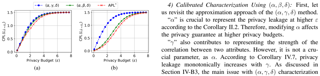
Figures from the paper (8 more)


Reference graph
Works this paper leans on
-
[14]
The Hidden Cost of Correlation: Rethinking Privacy Leakage in Local Differential Privacy
S. Jayawardana, S. Ulukus, M. Ding, and K. Thilakarathna, “The hidden cost of correlation: Rethinking privacy leakage in local differential privacy,” 2025. [Online]. Available: https://arxiv.org/abs/2508.12539
work page Pith review arXiv 2025
-
[26]
Quantifying differential privacy under temporal correlations,
Y . Cao, M. Yoshikawa, Y . Xiao, and L. Xiong, “Quantifying differential privacy under temporal correlations,” inICDE, 2017, pp. 821–832
work page 2017
-
[1]
Rappor: Randomized aggre- gatable privacy-preserving ordinal response,
U. Erlingsson, V . Pihur, and A. Korolova, “Rappor: Randomized aggre- gatable privacy-preserving ordinal response,” inProceedings of the 2014 ACM SIGSAC CCS, 2014
work page 2014
-
[2]
L-srr: Local differential privacy for location-based services with staircase randomized response,
H. Wang, H. Hong, L. Xiong, Z. Qin, and Y . Hong, “L-srr: Local differential privacy for location-based services with staircase randomized response,” in2022 ACM SIGSAC, ser. CCS ’22, p. 2809–2823
-
[3]
J. W. Kim, K. Edemacu, J. S. Kim, Y . D. Chung, and B. Jang, “A survey of differential privacy-based techniques and their applicability to location-based services,”Computers Security, vol. 111, 2021
work page 2021
-
[4]
PCKV: Locally differentially private correlated Key-Value data collection with optimized utility,
X. Gu, M. Li, Y . Cheng, L. Xiong, and Y . Cao, “PCKV: Locally differentially private correlated Key-Value data collection with optimized utility,” inUSENIX Security 20, 2020
work page 2020
-
[5]
Local differential privacy and its applications: A comprehensive survey,
M. Yang, T. Guo, T. Zhu, I. Tjuawinata, J. Zhao, and K.-Y . Lam, “Local differential privacy and its applications: A comprehensive survey,” Computer Standards Interfaces, 2024
work page 2024
-
[6]
Data privacy laws and their impact on financial technology companies: A review,
A. T. Oyewole, B. B. Oguejiofor, N. E. Eneh, C. U. Akpuokwe, and S. S. Bakare, “Data privacy laws and their impact on financial technology companies: A review,”Computer Science & IT Research Journal, 2024
work page 2024
Show all 50 references
-
[7]
Securema: protecting participant privacy in genetic association meta-analysis,
W. Xie, M. Kantarcioglu, W. S. Bush, D. C. Crawford, J. C. Denny, R. Heatherly, and B. A. Malin, “Securema: protecting participant privacy in genetic association meta-analysis,”Bioinformatics, vol. 30 23, pp. 3334–41, 2014
2014
-
[8]
Local privacy and statistical minimax rates,
J. C. Duchi, M. I. Jordan, and M. J. Wainwright, “Local privacy and statistical minimax rates,” in2013 51st Annual Allerton Conference on Communication, Control, and Computing, 2013, pp. 1592–1592
2013
-
[9]
Privacy at scale: Local differential privacy in practice,
G. Cormode, S. Jha, T. Kulkarni, N. Li, D. Srivastava, and T. Wang, “Privacy at scale: Local differential privacy in practice,” ser. SIGMOD ’18. ACM, 2018, p. 1655–1658
2018
-
[10]
Collecting telemetry data privately,
B. Ding, J. Kulkarni, and S. Yekhanin, “Collecting telemetry data privately,” ser. NIPS’17, Red Hook, NY , USA, 2017, p. 3574–3583
2017
-
[11]
Learning with privacy at scale,
A. Inc., “Learning with privacy at scale,” https://machinelearning.apple. com/research/learning-with-privacy-at-scale, 2017
2017
-
[12]
Calm: Consistent adaptive local marginal for marginal release under local differential pri- vacy,
Z. Zhang, T. Wang, N. Li, S. He, and J. Chen, “Calm: Consistent adaptive local marginal for marginal release under local differential pri- vacy,” inACM SIGSAC Conference on Computer and Communications Security, ser. CCS ’18, 2018, p. 212–229
2018
-
[13]
No free lunch in data privacy,
D. Kifer and A. Machanavajjhala, “No free lunch in data privacy,” ser. SIGMOD ’11. ACM, 2011, p. 193–204
2011
-
[15]
On the risks of collecting multidimensional data under local differential privacy,
H. H. Arcolezi, S. Gambs, J.-F. Couchot, and C. Palamidessi, “On the risks of collecting multidimensional data under local differential privacy,”Proc. VLDB Endow., vol. 16, no. 5, p. 1126–1139, 2023
2023
-
[16]
Random sampling plus fake data: Multidimensional frequency estimates with local differential privacy,
H. H. Arcolezi, J.-F. Couchot, B. Al Bouna, and X. Xiao, “Random sampling plus fake data: Multidimensional frequency estimates with local differential privacy,” inProceedings of the 30th ACM CIKM, 2021, p. 47–57
2021
-
[17]
Impact of prior knowledge and data correlation on privacy leakage: A unified analysis,
Y . Li, X. Ren, S. Yang, and X. Yang, “Impact of prior knowledge and data correlation on privacy leakage: A unified analysis,”IEEE Transactions on Information Forensics and Security, vol. 14, no. 9, pp. 2342–2357, 2019
2019
-
[18]
Collecting high-dimensional and correlation-constrained data with local differential privacy,
R. Du, Q. Ye, Y . Fu, and H. Hu, “Collecting high-dimensional and correlation-constrained data with local differential privacy,” in2021 18th Annual IEEE SECON, 2021, pp. 1–9
2021
-
[19]
Aaa: An adaptive mechanism for locally differentially private mean estimation,
F. Wei, E. Bao, X. Xiao, Y . Yang, and B. Ding, “Aaa: An adaptive mechanism for locally differentially private mean estimation,”Proc. VLDB Endow., vol. 17, no. 8, p. 1843–1855, 2024
2024
-
[20]
Local differential privacy for correlated location data release in its,
K. M. Chong and A. Malip, “Local differential privacy for correlated location data release in its,”Computer Networks, vol. 255, p. 110830, 2024
2024
-
[21]
Correlated differential privacy: Hiding information in non-iid data set,
T. Zhu, P. Xiong, G. Li, and W. Zhou, “Correlated differential privacy: Hiding information in non-iid data set,”IEEE Transactions on Informa- tion Forensics and Security, vol. 10, no. 2, pp. 229–242, 2015
2015
-
[22]
T. M. Cover and J. A. Thomas,Entropy, Relative Entropy, and Mutual Information. John Wiley and Sons, Ltd, 2005, ch. 2, pp. 13–55. [Online]. Available: https://onlinelibrary.wiley.com/doi/abs/10. 1002/047174882X.ch2
2005
-
[23]
User’s guide to correlation coefficients,
H. Akoglu, “User’s guide to correlation coefficients,”Turkish Journal of Emergency Medicine, vol. 18, no. 3, pp. 91–93, 2018
2018
-
[24]
Locally differentially private frequent itemset mining,
T. Wang, N. Li, and S. Jha, “Locally differentially private frequent itemset mining,” in2018 IEEE Symposium on Security and Privacy (SP), 2018, pp. 127–143
2018
-
[25]
The staircase mechanism in differential privacy,
Q. Geng, P. Kairouz, S. Oh, and P. Viswanath, “The staircase mechanism in differential privacy,”IEEE Journal of Selected Topics in Signal Processing, vol. 9, pp. 1176–1184, 2015
2015
-
[27]
Locally differentially private protocols for frequency estimation,
T. Wang, J. Blocki, N. Li, and S. Jha, “Locally differentially private protocols for frequency estimation,” inUSENIX Security 17, 2017, pp. 729–745
2017
-
[28]
ACS Supplemental Poverty Measure (SPM) Research Files: 2009–2019, 2021–2023,
U.S. Census Bureau, “ACS Supplemental Poverty Measure (SPM) Research Files: 2009–2019, 2021–2023,” https://www.census. gov/data/datasets/time-series/demo/supplemental-poverty-measure/ acs-research-files.html, 2025
2009
-
[29]
Dss 2016 dataset,
A. U. R. I. N. (AURIN), “Dss 2016 dataset,” https://data.gov.au/data/ dataset/dss-payment-demographic-data
2016
-
[30]
A comprehensive survey on local differential privacy toward data statistics and analysis,
T. Wang, X. Zhang, J. Feng, and X. Yang, “A comprehensive survey on local differential privacy toward data statistics and analysis,”Sensors, vol. 20, no. 24, 2020
2020
-
[31]
Computability of global solutions to factorable nonconvex programs: Part i—convex underestimating problems,
G. P. McCormick, “Computability of global solutions to factorable nonconvex programs: Part i—convex underestimating problems,”Math- ematical Programming, vol. 10, no. 1, pp. 147–175, 1976
1976
-
[32]
Boyd and L
S. Boyd and L. Vandenberghe,Convex Optimization. Cambridge University Press, 2004
2004
-
[33]
Deep learning face attributes in the wild,
Z. Liu, P. Luo, X. Wang, and X. Tang, “Deep learning face attributes in the wild,” inICCV, December 2015
2015
-
[34]
Becker and R
B. Becker and R. Kohavi, “Adult,” UCI Machine Learning Repository, 1996, DOI: https://doi.org/10.24432/C5XW20
1996 doi
-
[35]
Cardiovascular disease dataset,
S. Sulianova, “Cardiovascular disease dataset,” https://www.kaggle.com/ datasets/sulianova/cardiovascular-disease-dataset, 2021
2021
-
[36]
Macro f1 and macro f1,
J. Opitz and S. Burst, “Macro f1 and macro f1,” 2021. [Online]. Available: https://arxiv.org/abs/1911.03347
2021 arXiv
-
[37]
The theory of decision procedures for distri- butions with monotone likelihood ratio,
S. Karlin and H. Rubin, “The theory of decision procedures for distri- butions with monotone likelihood ratio,”The Annals of Mathematical Statistics, vol. 27, pp. 272–299, 1956
1956
-
[38]
Differential privacy,
C. Dwork, “Differential privacy,” inAutomata, Languages and Program- ming, M. Bugliesi, B. Preneel, V . Sassone, and I. Wegener, Eds. Berlin, Heidelberg: Springer Berlin Heidelberg, 2006, pp. 1–12
2006
-
[39]
Achieving k-anonymity privacy protection using gener- alization and suppression,
L. Sweeney, “Achieving k-anonymity privacy protection using gener- alization and suppression,”Int. J. Uncertain. Fuzziness Knowl.-Based Syst., vol. 10, no. 5, p. 571–588, Oct. 2002
2002
-
[40]
L-diversity: privacy beyond k-anonymity,
A. Machanavajjhala, J. Gehrke, D. Kifer, and M. Venkitasubramaniam, “L-diversity: privacy beyond k-anonymity,” inICDE’06, 2006, pp. 24– 24
2006
-
[41]
The algorithmic foundations of differential privacy,
C. Dwork and A. Roth, “The algorithmic foundations of differential privacy,”Foundations and Trends® in Theoretical Computer Science, vol. 9, pp. 211–407, 2014
2014
-
[42]
Enhancing correlated big data privacy using differential privacy and machine learning,
S. Biswas, A. Fole, N. Khare, and P. Agrawal, “Enhancing correlated big data privacy using differential privacy and machine learning,”Journal of Big Data, vol. 10, no. 1, p. 30, 2023
2023
-
[43]
Differentially private autocor- relation time-series data publishing based on sliding window,
J. Zhao, S. Liu, X. Xiong, and Z. Cai, “Differentially private autocor- relation time-series data publishing based on sliding window,”Secur. Commun. Networks, vol. 2021, pp. 6 665 984:1–6 665 984:10, 2021
2021
-
[44]
Ldp-based social content protection for trending topic recommendation,
J. Wei, J. Li, Y . Lin, and J. Zhang, “Ldp-based social content protection for trending topic recommendation,”IEEE IoT Journal, vol. 8, no. 6, pp. 4353–4372, 2021
2021
-
[45]
Tabtransformer: Tabular data modeling using contextual embeddings,
X. Huang, A. Khetan, M. Cvitkovic, and Z. Karnin, “Tabtransformer: Tabular data modeling using contextual embeddings,” 2020. [Online]. Available: https://arxiv.org/abs/2012.06678 APPENDIX OPENSCIENCE Artifacts are available in https://github.com/ SandaruJayawardana/dependency-...
2020 arXiv
-
[46]
Sinceα 1 ≥1andγ 1 ≥1, denominator is positive (i.e.,λ 1, λ2 >0)
+e α1 (eγ1 −1). Sinceα 1 ≥1andγ 1 ≥1, denominator is positive (i.e.,λ 1, λ2 >0). Therefore, if and only ifα 1 ≥γ 1 thenU 1 −U 2 ≥0. This completes the proof. APPENDIXE PROOF OFTHEOREMIV.3 Proof.Based on new constraints in (9), we can formulate the updated optimization problem ...
-
[47]
ComputeV ⋆:We check the valid value range ofg ′ and howV(·)behaves withg ′ for g= eγ +ˆδ+g ′−1 eγ and g=e αg′ + ˜δ. •If g= eγ +ˆδ+g ′−1 eγ then V(g ′, δ, ε, α) =1 +e −γ(eγ + ˆδ+g ′ −1)(e ε −1) 1 +g ′(eε −1) .(41) Sincee −γ(eε −1)−(e ε −1)(1 +e −γ(eγ + ˆδ−1)(e ε −1)) = −e−γ(eε ...
-
[48]
Ifg ′ ∈[0, eγ −1−˜δeγ +ˆδ eα+γ −1 ]then g=e αg′ + ˜δ
-
[49]
Furthermore,e αg′ + ˜δ= eγ +ˆδ+g ′−1 eγ atg ′ = eγ −1−˜δeγ +ˆδ eα+γ −1
Ifg ′ ∈[ eγ −1−˜δeγ +ˆδ eα+γ −1 ,1]then g= eγ +ˆδ+g ′−1 eγ . Furthermore,e αg′ + ˜δ= eγ +ˆδ+g ′−1 eγ atg ′ = eγ −1−˜δeγ +ˆδ eα+γ −1 . Therefore, we can computeV ⋆ based on the value of eγ −1−˜δeγ +ˆδ eα+γ −1 under three cases. Case 1 - ( eγ −1−˜δeγ +ˆδ eα+γ −1 ≤0)Sinceg ′ ≥0, ...
-
[50]
Interestingly, each of the above cases has attainableG andG ′
Optimality ofV ⋆:Next, let us evaluate the optimality ofV ⋆. Interestingly, each of the above cases has attainableG andG ′. For example, consider the case eγ −1− ˜δeγ + ˆδ eα+γ −1 ≤0. In this scenario, we selectG ′ i for alli∈[b]\Sas G′ i =e γGi + ˆδi, such that P i∈[b]\S G′ i...
Reviewed August 5, 2026 · model on record in the stance chip above.
Discussion (0). Sign in to comment.