REVIEW 4 major objections 5 minor 44 references
Distribution of the Radius of Gyration for an ISAW
T0 review · 4 major / 5 minor · reviewed 2026-08-10 · deepseek-v4-flash
Pith's one-line read The paper derives an explicit free energy as a function of the radius of gyration for an interacting self-avoiding walk, showing that the resulting distribution matches Monte Carlo histograms from coil to globule except at the immediate…
desk verdict A useful, honest phenomenological fit of the ISAW radius-of-gyration distribution, but the central formula is not derived and its validation is in-sample; worth refereeing with demands for out-of-sample tests. read the letter →
The pith
A machine-rendered reading of the paper's core claim, the machinery that carries it, and where it could break.
The reading
What carries the argument
The load-bearing object is the renormalized density $t = \rho^{g}$ with $g=1/(\nu d-1)$, built from the monomer density $\rho=N/R^d$ and the Flory exponent $\nu$. Matching the free energies of stretched, globular, and scale-invariant coil conformations fixes the exponents of the terms, and $t$ is the variable in which the low-density free energy is assumed analytic. The second piece is the cumulant expansion that expresses the interacting free energy as the non-interacting one minus the generating function of the contact-number cumulants $\kappa_n(t)$; the assumption that each $\kappa_n(t)=N(a_n+B_n t+B'_n t^2+o(t^2))$ is extensive and analytic in $t$ turns the infinite sum into the quadratic structure of Eq. (56). The surface term $(N t^2)^{(d-1)/d}$ is fixed by requiring both the crossover scaling $\hat t=N^{1/2}t$ and the $N^{(d-1)/d}$ dependence of a globule surface.
What would settle it
Measure, from the same fixed-$R$ contact-count histograms used in the paper, the third cumulant $\kappa_3(t)$ for a range of $N$ and $\varepsilon$ and test whether it follows $N(a_3+B_3 t+B_3' t^2)$ across the crossover. If it shows non-analytic behaviour in $t$ or an extra $N$-dependence, the general form Eq. (56) is falsified. A second, direct test is to fit the exponent of the quadratic term in $t$ from histograms taken in a narrow band around $\varepsilon_\Theta$; consistency with $\nu_\theta=1/2$ would demand an effective exponent of about 1.53 instead of 2, settling whether the $t^2$ term is truly universal.
Extended reading notes
Core claim
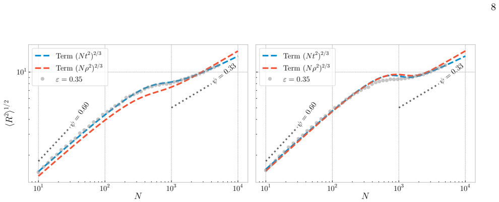
The central claim is that for a three-dimensional lattice ISAW the finite-size free energy as a function of the renormalized density $t=(N/R^3)^{1/(3\nu-1)}$ is $$\$\beta$ F_N(t|\varepsilon) = a_1(\varepsilon) N t + a_2(\varepsilon) N $t^{2}$ + a_3(\varepsilon) (N t)^{-q} + a_4(\varepsilon) (N $t^{2}$)^{2/3} + c_N(\varepsilon) \ln(N t),$$ with $c_N(\varepsilon)=c_0(\varepsilon)+c_1(\varepsilon)/N+c_2(\varepsilon)\ln N$. The radius-of-gyration distribution then follows from $P(R|\varepsilon,N) \propto \exp[-\beta F_N(t|\varepsilon)]$. The first two terms are the low-density virial-like expansion in $t$; the $(N t)^{-q}$ term and the logarithm encode entropic and surface counting corrections; the $(N t^2)^{2/3}$ term is a new surface-energy contribution chosen by scaling arguments. The paper validates the formula against Monte Carlo data for chain lengths from about 8 to 23,000 monomers and interaction strengths from 0 to 0.39, reporting agreement for the full histograms, means, and medians except in a narrow window at the immediate vicinity of the $\Theta$-point, and uses it to build a finite-$N$ coil-globule phase diagram.
Load-bearing premise
The derivation's load-bearing premise is that every cumulant of the contact-number distribution at fixed radius is extensive and analytic in the renormalized density $t$, with only linear and quadratic corrections to the leading $N$ term; anything more than that cannot be absorbed into the seven fitted coefficients without making Eq. (56) a fit rather than the claimed general expression.
Editorial extensions
If this is right
- For a lattice ISAW, the full finite-size distribution $P(R^2|\varepsilon,N)$ is available in closed form once the seven $\varepsilon$-dependent coefficients are known, without further simulation.
- A two-dimensional finite-$N$ phase diagram can be constructed from the inflection of the mean radius as a function of $N$; the phase boundary is consistent with $\varepsilon_N = a N^{-b} + \varepsilon_\Theta$ or with the classical $N^{-1/2}+N^{-1}$ form, with $\varepsilon_\Theta \approx 0.27$.
- The formula reproduces the mean, median, and entire histograms of $R^2$ for $N$ from roughly 8 to 23,000 and $\varepsilon$ from 0 to 0.39, which the paper takes as validating the factorized $N$- and $\varepsilon$-dependence.
- Because the $\varepsilon$-dependence is contained entirely in the coefficients, the same free energy can be used to compare different chain lengths at a given solvent quality without refitting.
- The authors propose the expression as a basis for mapping off-lattice or coarse-grained polymer models onto the lattice ISAW description.
Reading between the lines
- If Eq. (56) is correct, the distribution itself supplies a likelihood function for estimating $\varepsilon$ from a single-molecule histogram of $R$, which is the only order parameter accessible in super-resolution imaging of chromatin or intrinsically disordered proteins.
- The fitted $a_4(\varepsilon)$ increasing toward $\varepsilon=0$ hints at parameter compensation; extrapolating the formula to $\varepsilon$ values outside the fitted range, or using the individual coefficients as physical virial coefficients, may therefore be unsafe.
- The unresolved contradiction between the quadratic $t^2$ term and the required $\nu_\theta=1/2$ at the $\Theta$-point suggests the true crossover variable may involve an effective exponent $n\simeq 1.53$; simulations at larger $N$ just above $\varepsilon_\Theta$ could settle which form is fundamental.
- The surface term $(N t^2)^{2/3}$ predicts a specific dependence on spatial dimension $d$ through $(N t^2)^{(d-1)/d}$; testing the formula in $d=2$ would discriminate it from earlier surface-energy forms.
Editorial analysis
A structured set of objections, weighed in public.
Referee Report
Summary. The paper claims to derive an explicit finite-size free energy for a three-dimensional interacting self-avoiding walk (ISAW) as a function of the radius of gyration, chain length N, and interaction energy ε. The central result is Eq. (56), βF_N(t|ε) = a1(ε) N t + a2(ε) N t^2 + a3(ε) (N t)^{-q} + a4(ε) (N t^2)^{2/3} + c_N(ε) ln N t, with t a renormalized density and c_N(ε) given by Eq. (53). The derivation proceeds through scaling arguments for the SAW free energy, a cumulant expansion of the contact-number distribution (Section IV), and ad hoc additions of logarithmic, stretched-chain, and surface terms (Section V). The seven ε-dependent coefficients are inferred by Bayesian MCMC from Monte Carlo simulations of lattice ISAWs, and the resulting distributions are compared with the same simulated histograms. The paper also uses the fitted formula to construct a finite-size coil-globule phase diagram.
Significance. If the central formula were established as a genuine free-energy expression, it would provide a compact, transferable description of the entire radius-of-gyration distribution across coil and globule regimes, with practical value for interpreting single-molecule and super-resolution experiments. The manuscript's strengths are its extensive lattice simulations (chain lengths up to ~23,000, many ε values), the transparency of the Bayesian inference procedure, and the provided reproducible code. However, the claimed derivation rests on unverified assumptions about the cumulants, the functional form is partly the outcome of trial-and-error model selection, and the validation is in-sample. These issues currently limit the result to a well-tested phenomenological fit rather than the explicit derived free energy advertised in the abstract and conclusions.
major comments (4)
- [Section IV.B, Eq. (37)] The central step of the derivation is the assertion that every contact-number cumulant κ_n(t) is extensive and has the analytic asymptotic form N(a_n + B_n t + B'_n t^2 + o(t^2)). This is stated for all orders n without proof or direct numerical check. Since Eqs. (41) and (56) inherit their t and t^2 dependence from this assumption, the claimed generality of the free-energy formula is not established. The paper itself notes in Section VI.D that consistency with the known Θ-point exponent ν_θ = 1/2 would replace the t^2 term by t^n with n ≈ 1.53, explicitly acknowledging that the exponent 2 is not universal. The authors should either derive the cumulant expansion from a controlled approximation, or directly measure κ_n(t) from the simulations at fixed R and test Eq. (37).
- [Section V.A–V.B, Eqs. (51)–(56)] The logarithmic term c_N(ε) ln N t, the stretched-chain term (N t)^{-q}, and the surface term (N t^2)^{2/3} are introduced through "careful trial and error" and "several trials" after poor fits, rather than derived. The exponent q is never defined, estimated, or reported, so Eq. (56) is not an explicit closed-form free energy in the sense claimed. At minimum, q must be specified and the derivation of the surface term's exponent should be made independent of the fitting data, or the manuscript should be reframed as presenting a phenomenological free-energy form.
- [Section VI.B–VI.D] The validation is circular. The parameter vector θ(ε) = (a1, a2, a3, a4, c0, c1, c2) is obtained by maximizing the likelihood in Eq. (57) over the same {R^2_i,N} histograms that are later compared with the theory in Figures 2–5. With seven parameters per ε and additional piecewise polynomial regressions in ε (Section VI.C), the agreement measures the quality of the fit, not the predictive validity of Eq. (56). To support the abstract's claim that this "validates our resulting free energy expression," the authors should perform a held-out validation: fit θ(ε) on one subset of the (N, ε) grid and compare predictions on the complementary subset, or use k-fold cross-validation.
- [Section VI.C] The authors report that a4 unreasonably increases as ε → 0 and attribute this to "overfitting in these conditions." This admission indicates that the fitted coefficients can compensate for missing or misspecified terms in Eq. (56). Consequently, the physical interpretation of a1(ε) as the second virial coefficient and of other coefficients as specific free-energy contributions is not uniquely supported: equally good fits might be obtained with different term balances. The claim that the parameters have "a clear interpretation" (Section VII) therefore needs additional support, for example by checking the stability of each a_i(ε) when terms are removed one at a time.
minor comments (5)
- [Section V.A, Eq. (51)] The exponent q in the term (N t)^{-q} is left undefined in the text and never estimated; please state its value, or at minimum how it is determined, since it is part of the central formula.
- [Section VI.E] The phrase "infection point" should be "inflection point".
- [References] Reference [21] gives the publisher of de Gennes' book as "Cornel University Press"; this should be "Cornell University Press".
- [Section VI.D] The explanation that the discrepancy at ε = 0.28 is "numerical rather than theoretical" is speculative and not tested (e.g., by longer simulations or different equilibration protocols); since the parameters are fitted to the same data, the deviation could equally indicate missing terms in Eq. (56).
- [Section III, Eqs. (8)–(11)] The matching conditions are presented as if they determine the free-energy exponents uniquely, but the derivation assumes power-law forms for S, G, and C without justifying why sums of only two power laws are sufficient; a sentence acknowledging this modeling assumption would improve clarity.
Circularity Check
The claimed validation of Eq. (56) is an in-sample fit: the seven parameters θ(ε) are inferred from the same R² histograms that are later called 'theoretical predictions', and part of the functional form (logarithmic and surface terms) was chosen by trial and error against those same simulations.
-
fitted input called prediction
[Section VI.B, Eq. (57), and Section VI.D]
"We build the probability density function for R^2, P(R^2|ε,N), using the explicit free energy Equation (56) and maximizing the log-likelihood function L(θ(ε))≡ln ∏_{i,N} P(R^2_{i,N}|ε,N) ... We assess a posteriori the quality of the free energy expression and of the resulting parameters θ(ε) = (a1, a2, a3, a4, c0, c1, c2) by comparing the theoretical predictions - obtained from (15) and (56) using the Bayesian estimates of θ(ε) - to the simulated distributions of R^2."
The parameters θ(ε) are obtained by maximizing the log-likelihood over the same {R^2_{i,N}} dataset that is later used for the 'theoretical predictions' comparison in Section VI.D. The theoretical curves are therefore the fitted model evaluated at its best-fit parameters, and the agreement is an in-sample goodness-of-fit measure. The comparison is forced to be favorable by construction and cannot independently validate Eq. (56) as a prediction.
-
fitted input called prediction
[Section V.B, after Eq. (56)]
"In summary, we derived an explicit formula for the free energy, Equation (56), including a surface term and a modified logarithmic term, both of which were fitted using extensive simulations."
The text explicitly states that two terms of the central free energy, Eq. (56), were fitted using the same extensive Monte Carlo simulations that later serve as the validation data. Earlier in Section V.A, the logarithmic correction was introduced by 'a careful trial and error steps' to improve agreement with those simulations, and the surface term was adopted after comparing with the same data. Thus the functional form of the 'derived' free energy is partly selected on the validation set, so the subsequent agreement with the histograms reduces to an in-sample model-selection result rather than an independent test of the derivation.
full rationale
The non-interacting SAW part and the cumulant-expansion scaffolding (Eqs. 22–31) are not circular in themselves: they are exact identities or scaling postulates, and the t = ρ^g variable has an independent matching-conditions argument. However, the paper's central deliverable, Eq. (56), is not a parameter-free first-principles result: its coefficients θ(ε) are maximum-likelihood estimates on the same {R^2} histograms to which the formula is then compared, and part of its functional form (the c_N ln term and the surface term) was selected by trial and error against those same simulations. The abstract/conclusion phrase 'This validates our resulting free energy expression' is therefore an in-sample fit assessment, not an external test. I did not count the self-citations to Lhuillier, Victor and Imbert as circular per se: they are prior methodological references, and the scaling argument for t is reproduced in the text. I also note, as a non-circular correctness risk, that the t^2 term rests on the unverified all-orders extensivity/analyticity ansatz Eq. (37), which the paper itself undermines by reporting that Θ-point consistency would require exponent n ≈ 1.53 rather than 2; this weakens the derivation but does not by itself make it circular. Overall: partial circularity, score 6.
Assumptions & free parameters
free parameters (4)
- a1(ε), a2(ε), a3(ε), a4(ε), c0(ε), c1(ε), c2(ε) =
Bayesian posterior estimates at each of ~40 ε values; interpolation polynomials shown in Fig. 4
- q in the term (N t)^(-q) =
not stated in the text
- Polynomial regression coefficients for a_i(ε) and c_i(ε) =
not reported numerically
- ε_Θ (theta-point) =
≈0.28 from the a1(ε) crossing; 0.2703±0.0002 or 0.2719±0.0003 from phase diagram fits
assumptions (5)
- domain assumption The free energy of stretched, globular, and coil conformation classes is extensive and well described by power laws S(λ)=A_S λ^s, G(ρ)=A_G ρ^g, C(ϕ)=A_S ϕ^{c_s}+A_G ϕ^{c_g}.
- domain assumption βF(t|0,N) is analytic in t=ρ^g near t=0, so it admits the expansion A_G t + A'_G t^2 + o(t^2).
- ad hoc to paper All contact-number cumulants κ_n(t) are extensive and have the analytic asymptotic form N(a_n + B_n t + B'_n t^2 + o(t^2)).
- ad hoc to paper The truncated form with terms (N t)^(-q), (N t^2)^(2/3), and c_N(ε) ln N t captures the full free energy for all t, ε, N.
- ad hoc to paper a1(ε) vanishes linearly near ε_Θ, i.e., a1(ε) ∝ ε − ε_Θ.
Cite this review
Pith. "Pith review of Distribution of the Radius of Gyration for an ISAW." pith.science (2026). https://pith.science/paper/4JLSIOSY
@misc{pith2026260807195,
  author       = {Pith},
  title        = {Pith review of: Distribution of the Radius of Gyration for an ISAW},
  year         = {2026},
  howpublished = {\url{https://pith.science/paper/4JLSIOSY}},
  note         = {Machine review of arXiv:2608.07195}
}
abstract
We aim at calculating an explicit expression for the finite-size probability distribution of the radius of gyration $R$ of an Interacting Self-Avoiding Walk (ISAW), as a function of chain length $N$ and monomer-monomer interaction energy $\varepsilon$. We first derive the explicit free energy expression for a non-interacting Self-Avoiding Walk, introducing a new natural scale variable $t = \rho^g$ expressed as a power of the density $\rho$. Then, thanks to a cumulant expansion approach introduced by Lhuillier, Victor and coworkers, we extend it to the interacting case, capturing both the coil-globule transition and finite-size corrections to scaling, including entropic and surface-energy contributions. The radius of gyration distribution determined by the new free energy expression is then compared, using Bayesian inference to estimate the model parameters, to results from extensive Monte Carlo simulations of three-dimensional ISAWs, showing excellent agreement except very close to the $\Theta$-point, where finite chain lengths limit the accessible scaling regime. This validates our resulting free energy expression and allows us, as an application, to construct a phase diagram of the coil-globule transition.
Figures


Figures from the paper (3 more)


Reference graph
Works this paper leans on
-
[1]
O. Tochiyama, Y. Niibori, K. Tanaka, T. Kubota, H. Yoshino, A. Kirishima, and B. Setiawan, Modeling of the complex formation of metal ions with humic acids, Radiochimica Acta92, 10.1524/ract.92.9.559.54996 (2004)
-
[2]
A. Dobrynin, Theory and simulations of charged poly- mers: From solution properties to polymeric nanomate- rials, Current Opinion in Colloid & Interface Science13, 376 (2008)
work page 2008
- [3]
-
[4]
A. Y. Grosberg and A. R. Khokhlov,Statistical Physics of Macromolecules, AIP series in polymers and complex materials (AIP Press, 1994)
work page 1994
-
[5]
A. J. Spakowitz, Polymer physics across scales: Modeling the multiscale behavior of functional soft materials and biological systems, The Journal of Chemical Physics151, 230902 (2019)
work page 2019
-
[6]
de Gennes, Collapse of a polymer chain in poor solvents, Journal de Physique Lettres36, 55 (1975)
P.-G. de Gennes, Collapse of a polymer chain in poor solvents, Journal de Physique Lettres36, 55 (1975)
work page 1975
- [7]
-
[8]
P. Grassberger and R. Hegger, Simulations of three- dimensionalθpolymers, The Journal of Chemical Physics 102, 6881 (1995)
work page 1995
Show all 44 references
-
[9]
A. N. Rissanou, S. H. Anastasiadis, and I. A. Bitsanis, Monte carlo study of the coil-to-globule transition of a model polymeric system, Journal of Polymer Science Part B: Polymer Physics44, 3651 (2006)
2006
-
[10]
Allahverdi, R
A. Allahverdi, R. Yang, N. Korolev, Y. Fan, C. A. Davey, C.-F. Liu, and L. Nordenski¨ old, The effects of histone h4 15 tail acetylations on cation-induced chromatin folding and self-association, Nucleic Acids Research39, 1680 (2010)
2010
-
[11]
J. B. Imbert and J. M. Victor, Beyond flory's theory: A computer aided phenomenology for polymers, Molecular Simulation16, 399 (1996)
1996
-
[12]
J. B. Imbert, A. Lesne, and J. M. Victor, Distribution of the order parameter of the coil-globule transition, Phys- ical Review E56, 5630 (1997)
1997
-
[13]
Lhuillier, A simple model for polymeric fractals in a good solvent and an improved version of the flory ap- proximation, Journal de Physique49, 705 (1988)
D. Lhuillier, A simple model for polymeric fractals in a good solvent and an improved version of the flory ap- proximation, Journal de Physique49, 705 (1988)
1988
-
[14]
J. M. Victor and D. Lhuillier, The gyration radius distri- bution of two-dimensional polymer chains in a good sol- vent, The Journal of Chemical Physics92, 1362 (1990)
1990
-
[15]
Victor, J.-B
J.-M. Victor, J.-B. Imbert, and D. Lhuillier, The number of contacts in a self-avoiding walk of variable radius of gyration in two and three dimensions, The Journal of Chemical Physics100, 5372 (1994)
1994
-
[16]
Orland, Flory theory revisited, Journal de Physique I 4, 101 (1994)
H. Orland, Flory theory revisited, Journal de Physique I 4, 101 (1994)
1994
-
[17]
Nishio, S.-T
I. Nishio, S.-T. Sun, G. Swislow, and T. Tanaka, First ob- servation of the coil–globule transition in a single polymer chain, Nature281, 208 (1979)
1979
-
[19]
des Cloizeaux and G
J. des Cloizeaux and G. Jannink,Polymers in solution. Their modelling and structure(Oxford university press, New York, 1991)
1991
-
[20]
F¨ oldes, A
T. F¨ oldes, A. Lesage, and M. Barbi, Assessing the polymer coil-globule state from the very first spec- tral modes, Physical Review Letters127, 10.1103/phys- revlett.127.277801 (2021)
2021 doi
-
[21]
de Gennes,Scaling concepts in polymer physics (Cornel University Press, 1979)
P.-G. de Gennes,Scaling concepts in polymer physics (Cornel University Press, 1979)
1979
-
[22]
T. D. Lee and C. N. Yang, Statistical theory of equations of state and phase transitions. I. theory of condensation, Physical Review87, 404 (1952)
1952
-
[23]
Rodr ´ ıguez and C
A. Rodr ´ ıguez and C. Tsallis, A generalization of the cu- mulant expansion. application to a scale-invariant prob- abilistic model, Journal of Mathematical Physics51, 073301 (2010)
2010
-
[24]
A. L. Owczarek, T. Prellberg, and R. Brak, New scaling form for the collapsed polymer phase, Physical Review Letters70, 951 (1993)
1993
-
[25]
I. M. Lifshitz, A. Y. Grosberg, and A. R. Khokhlov, Some problems of the statistical physics of polymer chains with volume interaction, Reviews of Modern Physics50, 683 (1978)
1978
-
[26]
Khokhlov, Theory of the polymer chain collapse for the d-dimensional case, Physica A: Statistical Mechanics and its Applications105, 357 (1981)
A. Khokhlov, Theory of the polymer chain collapse for the d-dimensional case, Physica A: Statistical Mechanics and its Applications105, 357 (1981)
1981
-
[27]
Schnabel and W
S. Schnabel and W. Janke, Fast simulation of a large polymer with untruncated interaction near the collapse transition, Journal of Physics: Conference Series2241, 012005 (2022)
2022
-
[28]
Grassberger, Pruned-enriched rosenbluth method: Simulations ofθpolymers of chain length up to 1 000 000, Phys
P. Grassberger, Pruned-enriched rosenbluth method: Simulations ofθpolymers of chain length up to 1 000 000, Phys. Rev. E56, 3682 (1997)
1997
-
[29]
M. C. Tesi, E. J. J. van Rensburg, E. Orlandini, and S. G. Whittington, Monte carlo study of the interacting self-avoiding walk model in three dimensions, Journal of Statistical Physics82, 155 (1996)
1996
-
[30]
F. T. Wall and F. Mandel, Macromolecular dimensions obtained by an efficient monte carlo method without sam- ple attrition, The Journal of Chemical Physics63, 4592 (1975)
1975
-
[31]
Lal, ‘monte carlo’ computer simulation of chain molecules
M. Lal, ‘monte carlo’ computer simulation of chain molecules. i, Molecular Physics17, 57 (1969)
1969
-
[32]
Foreman-Mackey, D
D. Foreman-Mackey, D. W. Hogg, D. Lang, and J. Good- man, emcee: The MCMC hammer, Publications of the Astronomical Society of the Pacific125, 306 (2013)
2013
-
[33]
We used the Bayesian procedure described in the meth- ods section and applied it to each different value of the energy parameterε
for an example), defines the crossover region [8]. We used the Bayesian procedure described in the meth- ods section and applied it to each different value of the energy parameterε. We were able to obtain the best estimates for each of the parametersa i(ε),c i(ε). The results ...
-
[34]
Lesage, V
A. Lesage, V. Dahirel, J.-M. Victor, and M. Barbi, Poly- mer coil–globule phase transition is a universal folding principle of drosophila epigenetic domains, Epigenetics & Chromatin12, 10.1186/s13072-019-0269-6 (2019)
2019 doi
-
[35]
Wang, 50th anniversary perspective: Polymer con- formation—a pedagogical review, Macromolecules50, 9073 (2017)
Z.-G. Wang, 50th anniversary perspective: Polymer con- formation—a pedagogical review, Macromolecules50, 9073 (2017)
2017
-
[36]
Rampf, K
F. Rampf, K. Binder, and W. Paul, The phase diagram of a single polymer chain: New insights from a new simula- tion method, Journal of Polymer Science Part B: Polymer Physics44, 2542 (2006)
2006
-
[37]
I. C. Sanchez, Phase transition behavior of the isolated polymer chain, Macromolecules12, 980 (1979)
1979
-
[38]
Hofmann, A
H. Hofmann, A. Soranno, A. Borgia, K. Gast, D. Net- tels, and B. Schuler, Polymer scaling laws of unfolded and intrinsically disordered proteins quantified with single-molecule spectroscopy, Proceedings of the National Academy of Sciences109, 16155 (2012)
2012
-
[39]
Vettorel, G
T. Vettorel, G. Besold, and K. Kremer, Fluctuating soft- sphere approach to coarse-graining of polymer models, Soft Matter6, 2282 (2010)
2010
-
[40]
D. F. Parsons and D. R. M. Williams, An off-lattice wang-landau study of the coil-globule and melting transi- tions of a flexible homopolymer, The Journal of Chemical Physics124, 221103 (2006)
2006
-
[41]
H. Wu, K. Song, W.-R. Chen, J. Song, L. Porcar, and Z. Wang, Size and shape fluctuations of ultrasoft col- loids, Physical Review Research3, 10.1103/physrevre- search.3.033271 (2021)
2021 doi
-
[42]
Soranno, Physical basis of the disorder-order tran- sition, Archives of Biochemistry and Biophysics685, 108305 (2020)
A. Soranno, Physical basis of the disorder-order tran- sition, Archives of Biochemistry and Biophysics685, 108305 (2020)
2020
-
[43]
Cortini, M
R. Cortini, M. Barbi, B. R. Car´ e, C. Lavelle, A. Lesne, J. Mozziconacci, and J.-M. Victor, The physics of epige- netics, Rev. Mod. Phys.88, 025002 (2016)
2016
-
[44]
A. N. Boettiger, B. Bintu, J. R. Moffitt, S. Wang, B. J. Beliveau, G. Fudenberg, M. Imakaev, L. A. Mirny, C. ting Wu, and X. Zhuang, Super-resolution imaging reveals distinct chromatin folding for different epigenetic states, Nature529, 418 (2016)
2016
-
[45]
D. I. Cattoni, A. M. C. Gizzi, M. Georgieva, M. D. Ste- fano, A. Valeri, D. Chamousset, C. Houbron, S. D´ ejardin, J.-B. Fiche, I. Gonz´ alez, J.-M. Chang, T. Sexton, M. A. Marti-Renom, F. Bantignies, G. Cavalli, and M. Noll- mann, Single-cell absolute contact probability dete...
2017 doi
Reviewed August 10, 2026 · model on record in the stance chip above.
Discussion (0). Continue with ORCID to comment.