REVIEW 3 major objections 6 minor 33 references
Machine Learning for Physical Simulation Challenge Results and Retrospective Analysis: Power Grid Use Case
T0 review · 3 major / 6 minor · reviewed 2026-08-16 · deepseek-v4-flash
Pith's one-line read The paper reports that the winning AI-augmented power-flow solver outscored the exact physical solver, 64.2% to 62.5%, on the competition's aggregate metric, and argues hybrid AI-physics simulators could eventually replace physical…
desk verdict A credible competition retrospective whose headline claim—AI beat the physical solver—doesn't survive a change in the scoring weights, but the evaluation infrastructure and leaderboard are worth taking seriously. read the letter →
The pith
A machine-rendered reading of the paper's core claim, the machinery that carries it, and where it could break.
The reading
What carries the argument
The load-bearing object is the competition's aggregate score: $Score = 0.3\,Score_{\mathrm{test}} + 0.3\,Score_{\mathrm{OOD}} + 0.4\,Score_{\mathrm{speed\text{-}up}}$, where each sub-score is built from per-metric thresholds that turn errors into 0/1/2-point bins, and the speed-up score is a Weibull curve $1-\exp(-(x/a)^b)$ with $b=1.7$ and $c=5$, so $a = c(-\ln 0.9)^{-1/b}$. This formula carries the entire ranking: because speed has the largest coefficient, a slow but exact solver starts at a large disadvantage, and a solver whose accuracy and physics compliance are merely near-perfect can overtake it with a moderate speed-up.
What would settle it
Recompute the published sub-scores with a lower speed weight, for example $\alpha_{\mathrm{speed}}=0.2$ and $\alpha_{\mathrm{test}}=\alpha_{\mathrm{OOD}}=0.4$. Using the reported values (winner's combined test+OOD sub-score about 1.91 and speed score 0.17; physical solver's test+OOD sub-score 2.0 and speed score 0.06), the physical solver scores 0.812 versus the winner's 0.799, reversing the headline result.
Extended reading notes
Core claim
The paper claims that the top-ranked hybrid solver—a GPU-parallel method combining a neural initializer for voltage angles with a preconditioned conjugate-gradient power-flow solve—achieved a global score of 64.2% ± 0.62, slightly above the physical solver baseline's 62.5%. The physical solver remains perfect on accuracy and on all eight physics-compliance checks; the winner's edge comes from the speed-up component (raw speed-up about 7.9x versus 3.77x for the security-analysis baseline), while its accuracy and physics scores are slightly below perfect. The paper states this result as evidence that hybrid approaches could replace physical solvers in the future, while acknowledging that scalability to real grids and generalization across configurations remain open.
Load-bearing premise
The load-bearing premise is the competition's choice to give speed 40% of the final score and accuracy on the test sets only 30% each; lower the speed weight below roughly 28% and the exact physical solver would rank first.
Editorial extensions
If this is right
- If the result holds, hybrid AI-physics solvers can serve as contingency screeners, reducing the number of full power-flow simulations needed for N-1 and N-2 risk analysis.
- Near-perfect physics compliance is achievable with hard constraints, such as zeroing disconnected-line outputs and projecting predictions onto local conservation laws, and these constraints also stabilize out-of-distribution behavior.
- The speed-up score saturates around a 30x acceleration, so the benchmark rewards practical throughput improvements without over-rewarding extreme speed.
- The paper's organizational conclusion is that retraining every finalist model on identical servers makes the comparison reproducible and fair, and that future editions should test scalability to larger grids.
Reading between the lines
- The 'outperforms physics' claim is a scoring artifact in a specific sense: the exact solver is still more accurate and more physics-compliant, and the winner's advantage comes from the speed component; if the speed weight drops below roughly 28%, the exact solver would rank first.
- Because the Weibull speed curve nearly saturates above about 30x speed-up, two systems with very different raw latencies could tie on the aggregate metric, so the leaderboard understates speed differences among the fastest methods.
- A natural next experiment is to rerun the same benchmark on a larger grid and on renewable penetration levels beyond 30%; the winner's hyper-sparse block-diagonal GPU approach plausibly scales, but the paper does not demonstrate it.
Signed reviews
Editorial analysis
A structured set of objections, weighed in public.
Referee Report
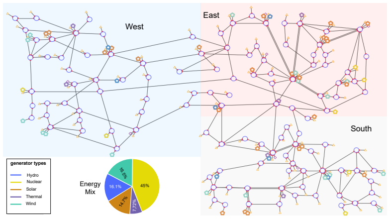
Summary. This paper reports the ML4PhySim competition for power-flow simulation on an IEEE 118-bus regional grid with roughly 30% renewable penetration (the L2RPN IDF 2023 environment). Participants submitted trainable models mapping injections and topology to line currents, powers, and voltages; finalists' code was retrained and evaluated on the organizers' standardized GPU servers within a 12-hour budget. Scoring aggregates ML accuracy (MAPE90, MAPE107, MAE), eight physics-compliance criteria (P1-P8), an out-of-distribution generalization set (double line disconnections unseen in training), and speed-up relative to LightSim2grid via Score = 0.3*Score_test + 0.3*Score_OOD + 0.4*Score_speed (Eq. (2)), with speed-up scored by a Weibull curve (Eq. (D.5), b = 1.7, c = 5); the final ranking uses 10 repeated runs. The winner, HyPowerFlow (ASU), is a GPU-parallel preconditioned-conjugate-gradient solver with an ML-initialized voltage-angle guess; second is LEAP-PINN (XJTU), a LEAPNet variant with KKT-based hard constraints; third is a cross-attention transformer (UToronto). The headline result is a winner's global score of 64.2 versus the physical-solver baseline's 62.5, stated as 'outperformed the physical solver.' The paper closes with organizational lessons on materials, incentives, and infrastructure.
Significance. If the headline result were robust, the paper would be a well-executed demonstration that ML-augmented simulators can run at substantial speed-ups on a realistic grid while passing a battery of physics-compliance checks, a meaningful signal for hybrid modeling in TSO operations. The competition design has genuine methodological strengths: pre-registered splits with fixed seeds, fully standardized GPU infrastructure, mandatory retraining of finalists' code on organizers' servers (which mitigates hardware and leakage confounds), 10 repeated runs for final rankings, a purpose-built OOD test set, and open starting kits and winner code. However, the central claim is conditional on the scoring convention of Eq. (2)/(D.1): the physical solver is perfect on all accuracy and physics criteria and falls behind only because speed-up carries a 40% weight under a hand-chosen Weibull curve; the winner's margin reverses if the speed weight drops below about 30%.
major comments (3)
- [§5, §3.3, Table 4, Eqs. (D.1)-(D.5)] The claim that the winning solution 'outperformed the physical solver performance' (§5) and 'has the potential to replace physical solvers' (§3.3) is an artifact of the 40% speed-up weight in Eq. (D.1) and of the hand-chosen Weibull parameters b = 1.7, c = 5 in Eq. (D.5). The physical solver is perfect on every ML and physics sub-score on the test and OOD sets (Appendix F.1); it trails only because its speed-up score is 0.06 at 3.77x. From Table 4, the 1.7-point margin (64.2 vs 62.5) decomposes into roughly +5.8 points from the speed component (0.4 * (0.204 - 0.06)) and roughly -4.1 points from accuracy, physics, and OOD; if the speed-up weight were reduced below about 30%, the physical solver would regain the lead, and with zero speed weight it would win by about 6.6 points. No sensitivity analysis over the alpha coefficients or over b and c is reported, and the acknowledgment in Section 4.3 that discretization hides real-valued differences does not address this dependence. I recommend rewording the conclusion to state that the winner scored highest under this competition's deliberately speed-weighted scoring, and reporting the ranking's sensitivity to the weights.
- [Table 3, §2.4, Appendix D] The leaderboard in Table 3 cannot be reproduced from the information given in the text. Applying Eqs. (D.1)-(D.3) to the winner's reported sub-scores (ML-test 0.66, physics-test 0.28, ML-OOD 0.66, physics-OOD 0.28, speed 0.17) gives Score_test = Score_OOD approximately 0.53 and a global score of roughly 0.39, not the reported 0.63; the same recomputation fails for XJTU (approximately 0.39 computed versus 0.58 reported) and for UToronto (approximately 0.31 versus 0.42). In addition, the Speed-up column shows a value of 1.03 for the MPData entry, which cannot be a Weibull score (bounded above by 1) and is inconsistent with the speed-up ratios in Table 4 if it is instead a ratio. The paper should state precisely what each column reports (e.g., whether the ML and physics entries are the scores of Eqs. (D.3)-(D.4) or proportions of 'great' results) and should provide a worked reproduction of at least one winner's full score, as it already does for LeapNet in Appendix F.2.
- [Abstract, §3.3, Table 4] The stated objective is acceleration by 'at least an order of magnitude while maintaining operational reliability,' but the winning solution achieves 7.87x, below that target, and the only entry above 10x (UToronto, 12.42x) has markedly degraded ML and physics scores. Under Eq. (D.5), even the target 10x speed-up earns a speed score of only about 0.29, so the scoring gives limited credit for meeting the stated goal. The paper should separate the claims 'highest aggregate score under the competition weighting' from 'met the order-of-magnitude acceleration target,' and should report the raw metric values (MAPE90, MAPE107, MAE per quantity, and the P1-P8 violation rates) rather than only the discretized colors in Table 4, so that operational accuracy at the reported speed-ups can be assessed independently of the chosen thresholds.
minor comments (6)
- [Eq. (1), §2.2] In the reactive-power balance of Eq. (1), the printed sign convention (0 = qk + Σ...) differs from the usual injection convention shown in Eq. (B.2); please verify the signs and state the adopted convention explicitly.
- [§3.1, §3.3, Table 4, Appendix F.2] The LEAPNet baseline global score is given as 37.69 in Section 3.1 but as 37.6 in Section 3.3, Table 4, and Appendix F.2; these numbers should be harmonized.
- [Table 3 caption] The caption says two submissions were eliminated, and the text says the Codabench third-place solution was eliminated, but the table shows two dash-ranked rows (both labeled MPData) plus a Kuldeep row also with a dash; please clarify which rows were eliminated and how their scores relate to the ranking.
- [Table 4 caption] Table 4 contains two physical-solver rows (LightSim2grid at 1.0x with 60.2, and Security analysis at 3.77x with 62.5); the caption should state explicitly which of them is the speed-up reference and which is the 'physical solver baseline' used in the headline comparison.
- [§2.4] MAPE90 and MAPE107 are defined only verbally ('10% highest percentile' for currents and '90% highest quantile' for active powers); exact definitions with equations would remove ambiguity about whether the largest errors are averaged directly or as percentages.
- [§2.3, §5] Typos to correct: 'scnenarios' in the Section 2.3 heading, 'whether samples with only reference topology' should read 'either samples', and 'contuinty' should read 'continuity' in Section 5.
Circularity Check
No load-bearing circularity; competition ranking is externally generated. Minor score reflects self-cited LIPS/LEAPNet and hand-chosen scoring weights, not an equation-level reduction.
full rationale
The paper's central result is the ML4PhySim leaderboard. That ranking was not derived by fitting the paper's own equations to the target: Section 2.4 states participants 'were required to submit untrained models, which were then fully retrained and evaluated on the organizers' servers,' and Table 4 reports ten-run averages (64.2±.62 for the winner). The winner-vs-solver comparison is therefore an externally measured outcome, not a prediction manufactured from the scoring formula. The global score in Eq. (D.1) is a weighted combination with alpha_test=30%, alpha_ood=30%, alpha_speed-up=40%, and the speed-up sub-score uses the hand-chosen Weibull curve (b=1.7, c=5); changing these weights could change the ranking. That is a robustness/arbitrariness concern, not circularity: the winner's sub-scores are measured values, and no equation in the paper is equivalent to its input by construction. The self-citations to LIPS [19] and LEAPNet [20] are present but not load-bearing: LIPS is the evaluation harness and LEAPNet is a baseline, and neither forces the winner's score. The score of 2 reflects only these minor, non-load-bearing self-citations; there is no self-definitional, fitted-input, uniqueness-importing, or ansatz-smuggling step.
Assumptions & free parameters
free parameters (9)
- alpha_test (test dataset weight) =
0.3
- alpha_ood (OOD dataset weight) =
0.3
- alpha_speedup (speed-up weight) =
0.4
- alpha_ML (machine learning sub-weight) =
0.66
- alpha_physics (physics compliance sub-weight) =
0.34
- Weibull speed-up score shape parameter b =
1.7
- Weibull speed-up score scale parameter c =
5
- Physics compliance discretization thresholds =
Inferior 1%, Superior 5% for P1-P5, P8; Inferior 5%, Superior 10% for P6, P7
- ML metric discretization thresholds =
MAPE thresholds 2% and 5%; MAE thresholds 0.2 and 0.5
assumptions (5)
- standard math The alternating current power flow equations (Kirchhoff, Ohm, Joule) are the correct physical model of the grid.
- domain assumption LightSim2grid provides exact ground truth power flow values for training and evaluation.
- domain assumption The IEEE 118-bus based L2RPN IDF 2023 grid with a 30% renewable energy mix is representative of a near-future regional French power grid.
- domain assumption The selected metrics (MAPE90, MAPE10, MAE, and the eight physics compliance criteria) adequately capture operational reliability of a surrogate model.
- domain assumption The random chronic selection with fixed seeds produces independent and representative training, validation, test, and OOD distributions.
Cite this review
Pith. "Pith review of Machine Learning for Physical Simulation Challenge Results and Retrospective Analysis: Power Grid Use Case." pith.science (2026). https://pith.science/paper/2AHJ4AUO
@misc{pith2026250501156,
  author       = {Pith},
  title        = {Pith review of: Machine Learning for Physical Simulation Challenge Results and Retrospective Analysis: Power Grid Use Case},
  year         = {2026},
  howpublished = {\url{https://pith.science/paper/2AHJ4AUO}},
  note         = {Machine review of arXiv:2505.01156}
}
read the original abstract
This paper addresses the growing computational challenges of power grid simulations, particularly with the increasing integration of renewable energy sources like wind and solar. As grid operators must analyze significantly more scenarios in near real-time to prevent failures and ensure stability, traditional physical-based simulations become computationally impractical. To tackle this, a competition was organized to develop AI-driven methods that accelerate power flow simulations by at least an order of magnitude while maintaining operational reliability. This competition utilized a regional-scale grid model with a 30\% renewable energy mix, mirroring the anticipated near-future composition of the French power grid. A key contribution of this work is through the use of LIPS (Learning Industrial Physical Systems), a benchmarking framework that evaluates solutions based on four critical dimensions: machine learning performance, physical compliance, industrial readiness, and generalization to out-of-distribution scenarios. The paper provides a comprehensive overview of the Machine Learning for Physical Simulation (ML4PhySim) competition, detailing the benchmark suite, analyzing top-performing solutions that outperformed traditional simulation methods, and sharing key organizational insights and best practices for running large-scale AI competitions. Given the promising results achieved, the study aims to inspire further research into more efficient, scalable, and sustainable power network simulation methodologies.
Figures


Figures from the paper (8 more)


Reference graph
Works this paper leans on
-
[1]
D. K. Molzahn, I. A. Hiskens, et al., A survey of relaxations and approx- imations of the power flow equations (2019)
work page 2019
- [2]
-
[3]
J. Tompson, K. Schlachter, P. Sprechmann, K. Perlin, Accelerating eulerian fluid simulation with convolutional networks, ArXiv: 1607.03597 (2016)
arXiv 2016
-
[4]
M. Kasim, D. Watson-Parris, L. Deaconu, S. Oliver, P. Hatfield, D. Froula, G. Gregori, M. Jarvis, S. Khatiwala, J. Korenaga, et al., Building high accuracy emulators for scientific simulations with deep neural architecture search, Machine Learning: Science and Technology 3 (1) (2021) 015013
work page 2021
-
[5]
LEAP nets for power grid perturbations
B. Donnot, B. Donon, I. Guyon, Z. Liu, A. Marot, P. Panciatici, M. Schoenauer, Leap nets for power grid perturbations, arXiv preprint arXiv:1908.08314 (2019)
work page Pith review arXiv 2019
-
[6]
R. Lam, A. Sanchez-Gonzalez, M. Willson, P. Wirnsberger, M. Fortunato, F. Alet, S. Ravuri, T. Ewalds, Z. Eaton-Rosen, W. Hu, et al., Learning skillful medium-range global weather forecasting, Science 382 (6677) (2023) 1416–1421. 44
work page 2023
- [7]
-
[8]
M. Yagoubi, D. Danan, M. Leyli-abadi, J.-P. Brunet, J. A. Mazari, F. Bon- net, maroua gmati, A. Farjallah, P. Cinnella, P. Gallinari, M. Schoenauer, NeurIPS 2024 ML4CFD competition: Harnessing machine learning for computational fluid dynamics in airfoil design, in: NeurIPS 2024 Com- petition Track, 2024. URL https://openreview.net/forum?id=5Vw8xOVVkS
work page 2024
Show all 33 references
-
[9]
Yagoubi, M
M. Yagoubi, M. Leyli-Abadi, D. Danan, J.-P. Brunet, J. A. Mazari, F. Bonnet, A. Farjallah, M. Schoenauer, P. Gallinari, Ml4physim: Ma- chine learning for physical simulations challenge (the airfoil design), arXiv preprint arXiv:2403.01623 (2024)
2024 arXiv
-
[10]
Marot, B
A. Marot, B. Donnot, C. Romero, B. Donon, M. Lerousseau, L. Veyrin- Forrer, I. Guyon, Learning to run a power network challenge for training topology controllers, Electric Power Systems Research 189 (2020) 106635
2020
-
[11]
Marot, B
A. Marot, B. Donnot, G. Dulac-Arnold, A. Kelly, A. O’Sullivan, J. Viebahn, M. Awad, I. Guyon, P. Panciatici, C. Romero, Learning to run a power network challenge: a retrospective analysis, in: NeurIPS 2020 Competition and Demonstration Track, PMLR, 2021, pp. 112–132
2020
-
[12]
Marot, B
A. Marot, B. Donnot, K. Chaouache, A. Kelly, Q. Huang, R.-R. Hossain, J. L. Cremer, Learning to run a power network with trust, Electric Power Systems Research 212 (2022) 108487
2022
-
[13]
Marot, A
A. Marot, A. Kelly, M. Naglic, V. Barbesant, J. Cremer, A. Stefanov, J. Viebahn, Perspectives on future power system control centers for energy transition, Journal of Modern Power Systems and Clean Energy 10 (2) (2022) 328–344
2022
-
[14]
Marot, A
A. Marot, A. Rozier, M. Dussartre, L. Crochepierre, B. Donnot, Towards an ai assistant for human grid operators, arXiv preprint arXiv:2012.02026 (2020)
2020 arXiv
-
[15]
Lightsim2grid, https://github.com/BDonnot/lightsim2grid. 45
-
[16]
Donnot, I
B. Donnot, I. Guyon, M. Schoenauer, A. Marot, P. Panciatici, Antici- pating contingengies in power grids using fast neural net screening, in: 2018 International Joint Conference on Neural Networks (IJCNN), IEEE, 2018, pp. 1–8
2018
-
[17]
I. Pena, C. B. Martinez-Anido, B.-M. Hodge, An extended ieee 118-bus test system with high renewable penetration, IEEE Transactions on Power Systems 33 (1) (2017) 281–289
2017
-
[18]
Grid2op, https://github.com/Grid2op/grid2op
-
[19]
Leyli-abadi, A
M. Leyli-abadi, A. Marot, J. Picault, D. Danan, M. Yagoubi, B. Donnot, S. Attoui, P. Dimitrov, A. Farjallah, C. Etienam, LIPS-learning industrial physical simulation benchmark suite, Advances in Neural Information Processing Systems 35 (2022) 28095–28109
2022
-
[20]
Donon, B
B. Donon, B. Donnot, I. Guyon, Z. Liu, A. Marot, P. Panciatici, M. Schoe- nauer, Leap nets for system identification and application to power systems, Neurocomputing 416 (2020) 316–327
2020
-
[21]
L. Zeng, S. G. Alawneh, S. A. Arefifar, Gpu-based sparse power flow studies with modified newton’s method, IEEE Access 9 (2021) 153226– 153239
2021
-
[22]
Zlatev, Computational methods for general sparse matrices, Vol
Z. Zlatev, Computational methods for general sparse matrices, Vol. 65, Springer Science & Business Media, 2013
2013
-
[23]
Zhang, M
Y. Zhang, M. Zhang, Y. Liu, S. Ma, S. Feng, Localized matrix factor- ization for recommendation based on matrix block diagonal forms, in: Proceedings of the 22nd international conference on World Wide Web, 2013, pp. 1511–1520
2013
-
[24]
Y. Zhou, H. Cheng, J. X. Yu, Graph clustering based on structural/at- tribute similarities, Proceedings of the VLDB Endowment 2 (1) (2009) 718–729
2009
-
[25]
Adabag, M
E. Adabag, M. Atal, W. Gerard, B. Plancher, Mpcgpu: Real-time nonlinear model predictive control through preconditioned conjugate gradient on the gpu, in: 2024 IEEE International Conference on Robotics and Automation (ICRA), IEEE, 2024, pp. 9787–9794. 46
2024
-
[26]
Stott, O
B. Stott, O. Alsac, Fast decoupled load flow, IEEE transactions on power apparatus and systems (3) (2007) 859–869
2007
-
[27]
Zhang, M
J. Zhang, M. Mittenbuehler, L. Razik, A. Benigni, Parallel simulation of power systems with high penetration of distributed generation using gpus and opencl, in: 2022 IEEE 13th International Symposium on Power Electronics for Distributed Generation Systems (PEDG), IEEE, 2022, pp. 1–6
2022
-
[28]
H. Chen, G. E. C. Flores, C. Li, Physics-informed neural networks with hard linear equality constraints, Computers & Chemical Engineering 189 (2024) 108764
2024
-
[29]
S. P. Boyd, L. Vandenberghe, Convex optimization, Cambridge university press, 2004
2004
-
[30]
Vaswani, N
A. Vaswani, N. Shazeer, N. Parmar, J. Uszkoreit, L. Jones, A. N. Gomez, L. Kaiser, I. Polosukhin, Attention is all you need, Advances in neural information processing systems 30 (2017)
2017
-
[31]
Gilain, P
A. Gilain, P. Aknin, C. Balan, P. Le Masson, M. Leyli-Abadi, B. Weil, Training as an affordable and powerful lever to stimulate the evolution dynamics of a newly designed technology platform at the frontier between academia and industry, Tech. rep. (2025)
2025
-
[32]
Plantec, P
Q. Plantec, P. Le Masson, B. Weil, Simultaneous discovery–invention in corporate r&d: Lessons from the crispr case, European Management Review (2024)
2024
-
[33]
H. F. Hamann, T. Brunschwiler, B. Gjorgiev, L. S. Martins, A. Puech, A. Varbella, J. Weiss, J. Bernabe-Moreno, A. B. Mass´ e, S. Choi, et al., A perspective on foundation models for the electric power grid, arXiv preprint arXiv:2407.09434 (2024). 47
2024 arXiv
Reviewed August 16, 2026 · model on record in the stance chip above.
Discussion (0). Continue with ORCID to comment.