REVIEW 3 major objections 5 minor 1 cited by
Discontinuity-aware Normal Integration for Generic Central Camera Models
T0 review · 3 major / 5 minor · reviewed 2026-08-06 · deepseek-v4-flash
Pith's one-line read Normal integration now handles depth jumps and any central camera
desk verdict A genuinely new planar-pair relation for normal integration with honest benchmarks, but the blanket accuracy claim does not survive curved surfaces. read the letter →
The pith
A machine-rendered reading of the paper's core claim, the machinery that carries it, and where it could break.
The reading
What carries the argument
The load-bearing object is the pairwise identity (2)--(3), built from the ray-direction map $\tau(u)=(\tau_x(u),\tau_y(u),1)^T$ of a central camera and the surface normal $n$. The identity follows from solving a $6\times 6$ linear system whose six unknowns are the displacement components from the subpixel midpoint $m$ to the two pixel points; the two non-trivial equations impose that the local planes are perpendicular to $n_a$ and $n_b$ and that they differ only by a scalar $z$-offset $\varepsilon_{b\to a}$. Around this identity the paper constructs an optimization: a log-depth change of variables (7), BiNI-style bilateral weights (10), a discontinuity-activation term $\beta^{(t)}_{b\to a}$ (16) that switches on the $\varepsilon$ terms only where the bilateral weights signal a one-sided jump, and a generalized multiplicative factor $\gamma_{b\to a} = \|u_b-u_a\|/\|\tau_b-\tau_a\| \, n_a^T\tau_a$ that the paper analyses and shows controls both equation weighting and the sharpness of the bilateral sigmoid.
What would settle it
Render a known smooth object (e.g., a sphere of varying radius) with a pinhole camera, compute normals from the mesh, then measure the mean absolute residual of equation (2) with $\alpha=0$ on the true depth map and compare it against the residual of the BiNI PDE (8) on the same data; the paper's claim predicts the new residual should be lower or comparable across curvatures, while a fixed planarity-identity residual that grows faster with curvature would falsify the claim. A second decisive check: run the method on a scene with a known step discontinuity of known height and verify that the estimated $\varepsilon_{b\to a}$ converges to the true jump rather than to a jump that merely minimizes depth error.
Extended reading notes
Core claim
The paper's central claim is the depth-coupling relation $z_a = \omega^\varepsilon_a \, \varepsilon_{b\to a} + \omega_{b\to a}\,z_b$ with $\omega^\varepsilon_a = n_{az}/(n_a^T\tau_a)$ and $\omega_{b\to a} = (n_a^T\tau_m \, n_b^T\tau_b)/(n_a^T\tau_a \, n_b^T\tau_m)$, derived from asking that the surface around each of two neighbouring pixels be a plane perpendicular to its normal and that the two planes differ only by a z-axis offset $\varepsilon_{b\to a}$ at a subpixel midpoint along the connecting ray. This equation turns normal integration into a large sparse linear system $Az=b$ in the depth unknowns, with the discontinuity terms in $b$ recovered by an iterative bilateral scheme. The paper claims this formulation is the first to directly handle generic central cameras, that it approximates the true depth-normal relationship more accurately than PDE discretizations, and that it reaches state-of-the-art mean absolute depth error on the DiLiGenT benchmark (for instance 4.72 mm on goblet versus 8.53 mm for BiNI), with near-perfect reconstruction when the true discontinuities are supplied.
Load-bearing premise
The identity assumes every pixel neighbourhood is exactly a plane perpendicular to the normal, and that the two planes at neighbouring pixels cut a single subpixel ray with only one z-axis offset; strongly curved surfaces violate this, and the paper's own measurements show the accuracy advantage disappears on the high-curvature buddha object (residual 0.90 vs 0.46 for BiNI).
Editorial extensions
If this is right
- One algorithm covers orthographic, ideal-pinhole, and lens-distorted central cameras; previous leading methods needed separate or undistorted formulations.
- Explicit discontinuity variables let the optimizer estimate jumps instead of only hedging against them with robust weights, and the oracle experiment shows that if those jumps are known, depth is recovered to roughly 0.01--0.11 mm MADE.
- The generalized $\gamma_{b\to a}$ analysis transfers the earlier BiNI factor from a numerical device to a geometrically meaningful weight that down-weights pixel pairs near occluding boundaries.
- On the standard benchmark the method reports best or second-best mean absolute depth error on eight of nine objects, including a four-fold reduction on the discontinuous goblet object.
- The formulation also yields a practical pre-check for input normals: pixels with $n^T\tau > 0$ are physically invalid and can be filtered before integration, which the noise experiments show removes most spike artifacts.
Reading between the lines
- The failure on the high-curvature buddha object is an implicit boundary of the planarity assumption; an extension could compose this linear coupling with a curvature-adaptive smoothness term, using the residual of (2) itself as a curvature detector.
- Because the relation depends only on per-pixel ray directions, one can test it with non-central ray sets (e.g., ray maps of axial or catadioptric cameras) even though the paper explicitly excludes them; if the identity still holds with per-pixel $\tau$, the method would generalize in a straightforward way.
- The $\tau_m$ degree of freedom, currently fixed at the midpoint, could be tuned per pixel pair as a denoising mechanism; the paper shows outlier spikes correlate with $\omega_{b\to a}$ far from 1 and that re-sampling $\lambda_m$ reduces them, which suggests a confidence-weighted variant.
- The formulation accuracy metric (residual on ground-truth depth) could be repurposed as a benchmark signal for learning-based normal estimators: a normal map is geometrically consistent with some piecewise-planar scene exactly when this residual is low.
Editorial analysis
A structured set of objections, weighed in public.
Referee Report
Summary. This paper proposes a discontinuity-aware normal integration method for generic central cameras. The core idea is a local planarity assumption: for neighboring pixels a and b and a subpixel location m between them, the surface is modeled as two plane segments perpendicular to the local normals, and the two tangent-plane intersections with the midpoint ray tau_m are assumed to be separated by a scalar offset eps_b->a along the camera z-axis. Solving the resulting 6x6 system of ray-direction and perpendicularity equations yields the pairwise depth relation z_a = omega_eps^a * eps_b->a + omega_b->a * z_b with coefficients omega_eps^a = n_az/(n_a^T tau_a) and omega_b->a = (n_a^T tau_m * n_b^T tau_b)/(n_a^T tau_a * n_b^T tau_m), which is exact for piecewise-planar scenes. Depth and discontinuities are recovered by iterating conjugate-gradient solves of a weighted least-squares problem in log-depth variables, using BiNI-style bilateral weights and a sigmoidal activation beta that selectively enables relative discontinuities alpha_b->a. The paper validates the approach on DiLiGenT: the formulation residual on ground-truth depth is one to two orders of magnitude smaller than BiNI's on 8 of 9 objects, MADE is best or second best on all 9 objects, and an oracle row with known discontinuities reaches 0.01-0.34 mm. Experiments with Brown-Conrady lens distortion, real-world normal maps, and DiLiGenT-MV, plus extensive ablations, are also reported.
Significance. I view the contribution as solid and, conditional on the points below, publishable. The derivation of (2)-(3) is transparent, parameter-free, and correct; the concise alternative derivation in Appendix A provides an independent check. The oracle experiment, once its protocol is specified, would provide strong validation of the geometric model. The experimental protocol is careful: the BiNI baseline is rerun with its official code, Kim et al.'s numbers are quoted from the original paper, and the paper is unusually honest about hyperparameter sensitivity (Appendix E), outlier preprocessing requirements (Appendix H), and the limited scope of the distorted-camera comparison (Sec. 4.4). The gamma_b->a analysis in Appendix B, separating the focal-length and n^T tau effects, is a genuine insight beyond the main result. The main risks are the scope of the accuracy claim and the attribution of benchmark gains to the smooth relation versus the discontinuity mechanism; both are addressable in revision without new algorithmic development.
major comments (3)
- [Sec. 4.3, Table 2] The 'Ours with known discontinuity values' row is the evidence for the claim in Sec. 3.2 that, given ground-truth discontinuities, the optimization would recover ground-truth depth 'with close-to-perfect accuracy,' but the paper never specifies how the ground-truth eps_b->a (or alpha_b->a) values are computed. Please state explicitly whether they are computed geometrically from the ground-truth mesh as the z-offset between the intersections of the two per-pixel tangent planes with the midpoint ray tau_m, or obtained by inverting (2) from ground-truth depths. Only the former protocol validates the geometric model; the latter would make the near-perfect oracle recovery (0.01-0.34 mm) a tautology by construction. The small but nonzero errors on harvest (0.34 mm), goblet (0.11 mm), and buddha (0.10 mm) suggest a geometric computation, but without a stated protocol the experiment cannot be interpreted.
- [Abstract, Sec. 4.2, Table 1] The blanket claim that Eq. (2)-(3) 'more accurately approximates the relation between depth and surface normals' is not uniform across the benchmark. On buddha, the highest-curvature object, the mean absolute residual is 0.90 +/- 0.91 versus BiNI's 0.457 +/- 0.921 (Table 1), and the relative-residual tables in Appendix G show larger standard deviations for the proposed method on buddha and pot1. The text in Sec. 4.2 acknowledges 'all but one object,' but the abstract, introduction, and conclusion repeat the unqualified claim, and curvature sensitivity is absent from the limitations list in Appendix J. I ask for (i) a qualified claim 'on 8 of 9 DiLiGenT objects,' and (ii) an analysis of the model error against local surface curvature (e.g., a synthetic curved-surface experiment or a residual-versus-curvature scatter plot) so the reader can see where the per-edge z-offset model degrades.
- [Sec. 4.3, Table 2] The headline gains on the two discontinuous objects come almost entirely from the discontinuity mechanism rather than the smooth-surface relation. With alpha_b->a identically 0 at 1200 iterations, the method is worse than BiNI on harvest (4.83 vs 1.84 mm) and only moderately better on goblet (6.56 vs 9.00 mm); with alpha computation, the same rows become 0.73 and 4.72 mm. Since the abstract attributes the state-of-the-art results to a more accurate approximation of the depth-normal relation, the main text should attribute the gains explicitly: the smooth relation provides broad but modest improvements on low-curvature objects, while the explicit eps model is what delivers the large improvement on discontinuous objects. The rows of Table 2 already contain this information; what is missing is an explicit statement in the text.
minor comments (5)
- [Appendix C] There is a sign inconsistency in the first paragraph: the terms n_a^T tau_m and n_b^T tau_m are said to be 'strictly positive for all but a single pixel,' whereas the visibility discussion in Sec. 3.1 requires n^T tau < 0 for these dot products, and the subsequent argument that omega_b->a is positive relies on the same terms being negative. The text should read 'strictly negative.'
- [Eq. (13), Sec. 3.3] The generalization gamma_b->a = ||u_b-u_a||/||tau_b-tau_a|| * n_a^T tau_a is derived for the pinhole case from the identity ||Delta u||/||Delta tau|| = f, but for generic central cameras it is a heuristic. Because gamma changes the effective weighting (Appendix B, Table 3), the distorted-camera experiments would benefit from a brief justification or an ablation of alternative normalizations.
- [Appendix B] Labeling the two findings as 'Proposition 1' and 'Proposition 2' overstates their status; they are empirical observations supported by the ablations in Table 3, and should be relabeled as observations or empirical findings.
- [Sec. 4.2] The residual comparison is performed only against BiNI; since Kim et al. is presented as a co-leading method, the text should state explicitly that no public implementation was available and that the quantitative 'more accurate than existing methods' phrasing in the abstract is therefore based on a comparison with BiNI only.
- [General] The paper does not mention code availability; given the number of hyperparameters (q, rho, k, lambda_m, eps_out) and the iterative scheme, releasing the implementation would substantially support reproducibility.
Circularity Check
No significant circularity: Eq. (2)-(3) is derived algebraically from the stated local-planarity system (1) with no fitted parameters, and the benchmark comparisons are external and falsifiable.
full rationale
The central derivation is self-contained. Equation (2) with coefficients (3) is obtained by solving the six-equation system (1) in Appendix A (Eqs. 17-20); all coefficients are computed from known normals and ray directions, so the depth-coupling relation is not fitted to the depth data it is later used to recover. The claim that this relation 'more accurately approximates the relation between depth and surface normals' is tested by computing the residual of both formulations on the ground-truth DiLiGenT log-depth map (Table 1) and on relative residuals (Tables 7-8), which is an external, falsifiable comparison rather than a consequence of construction. The oracle experiment (Table 2, 'known discontinuity values') would be tautological only if the epsilon values were computed by inverting Eq. (2); the paper does not specify how these values are obtained, but it also does not define them via that inversion, and the reported small but nonzero errors (0.01-0.11 mm) suggest the oracle is not a numerical identity. The iterative alpha update in Eq. (14) does invert Eq. (7), and the authors openly state that applying it to all pairs would make the objective evaluate to zero; they introduce the activation term beta (Eqs. 15-16) to avoid this collapse. This is an explicit alternating-optimization loop, not a hidden circular 'prediction'. Limitations flagged in Appendix J (requirement n_a^T tau_a < 0, non-central cameras, runtime, hyperparameter dependence) and the worse residual on the curved buddha object (Tables 1 and 7) concern correctness and generalizability, not circularity. Adopting BiNI's bilateral weighting scheme [7] is clearly attributed and is not a load-bearing proof element.
Assumptions & free parameters
free parameters (5)
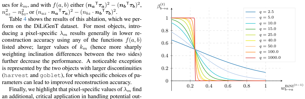
- q (discontinuity activation sharpness) =
50.0 (default; ablated 2.5 to 1000)
- rho (discontinuity activation threshold) =
0.25 (default)
- k (bilateral sigmoid sharpness) =
2 (BiNI default)
- lambda_m (subpixel ray parameter) =
0.5 (uniform midpoint)
- optimization iterations =
1200
assumptions (5)
- domain assumption Central camera model: every pixel ray originates at a single viewpoint and is represented by tau(u) = (tau_x(u), tau_y(u), 1); the surface is visible on a connected subset of the image plane with no inter-reflections.
- domain assumption Local planarity: each surface patch at a pixel is a plane perpendicular to the given normal, and the two planes of a neighbouring pair are related by a z-axis offset at the midpoint ray.
- domain assumption Visibility and validity of normals: for every pixel n_i^T tau_i < 0 and n_iz != 0, so omega_epsilon is defined and the log-depth reparametrization is valid.
- domain assumption Mid-ray positivity: with tau_m chosen as an interpolation of tau_a and tau_b, the terms n_a^T tau_m and n_b^T tau_m are negative, yielding omega_b_to_a > 0 and a defined logarithm in Eq. (7); positivity is then preserved by the alpha update.
- domain assumption Semi-smooth scenes: the surface has at most one-sided discontinuities per pixel, as assumed by BiNI's bilateral weighting scheme.
invented entities (1)
-
relative discontinuity field alpha_b_to_a = epsilon_b_to_a / z_b
Cite this review
Pith. "Pith review of Discontinuity-aware Normal Integration for Generic Central Camera Models." pith.science (2026). https://pith.science/paper/2VLL6XI5
@misc{pith2026250706075,
  author       = {Pith},
  title        = {Pith review of: Discontinuity-aware Normal Integration for Generic Central Camera Models},
  year         = {2026},
  howpublished = {\url{https://pith.science/paper/2VLL6XI5}},
  note         = {Machine review of arXiv:2507.06075}
}
read the original abstract
Recovering a 3D surface from its surface normal map, a problem known as normal integration, is a key component for photometric shape reconstruction techniques such as shape-from-shading and photometric stereo. The vast majority of existing approaches for normal integration handle only implicitly the presence of depth discontinuities and are limited to orthographic or ideal pinhole cameras. In this paper, we propose a novel formulation that allows modeling discontinuities explicitly and handling generic central cameras. Our key idea is based on a local planarity assumption, that we model through constraints between surface normals and ray directions. Compared to existing methods, our approach more accurately approximates the relation between depth and surface normals, achieves state-of-the-art results on the standard normal integration benchmark, and is the first to directly handle generic central camera models.
Figures


Figures from the paper (8 more)




Forward citations
Cited by 1 Pith paper
-
A Hybrid Neural-Microfacet BRDF Model for Real-Time Rendering
A hybrid BRDF model, combining a GGX analytical term with a tiny learned residual and gating network, fits measured materials more accurately than fully neural models at equal memory cost.
Reference graph
Works this paper leans on
-
[1]
An Algebraic Approach to Surface Reconstruction from Gradi- ent Fields
Amit Agrawal, Rama Chellappa, and Ramesh Raskar. An Algebraic Approach to Surface Reconstruction from Gradi- ent Fields. In ICCV, 2005. 1, 2
work page 2005
-
[2]
What Is the Range of Surface Reconstructions from a Gradient Field? In ECCV, 2006
Amit Agrawal, Ramesh Raskar, and Rama Chellappa. What Is the Range of Surface Reconstructions from a Gradient Field? In ECCV, 2006. 2
work page 2006
-
[3]
Ro- bust Surface Reconstruction via Triple Sparsity
Hicham Badri, Hussein Yahia, and Driss Aboutajdine. Ro- bust Surface Reconstruction via Triple Sparsity. In CVPR,
-
[4]
Gwangbin Bae and Andrew J. Davison. Rethinking Inductive 8 Biases for Surface Normal Estimation. In CVPR, 2024. 3, 6
work page 2024
-
[5]
Duane C. Brown. Decentering Distortion of Lenses. Pho- togrammetric Engineering, 32(3):444–462, 1966. 6
work page 1966
-
[6]
Normal Integration via Inverse Plane Fitting with Minimum Point-to-Plane Distance
Xu Cao, Boxin Shi, Fumio Okura, and Yasuyuki Matsushita. Normal Integration via Inverse Plane Fitting with Minimum Point-to-Plane Distance. In CVPR, 2021. 16
work page 2021
-
[7]
Xu Cao, Hiroaki Santo, Boxin Shi, Fumio Okura, and Ya- suyuki Matsushita. Bilateral Normal Integration. In ECCV,
-
[8]
Bilateral Normal Integration – Offi- cial implementation
Xu Cao, Hiroaki Santo, Boxin Shi, Fumio Okura, and Ya- suyuki Matsushita. Bilateral Normal Integration – Offi- cial implementation. https://github.com/xucao- 42/bilateral_normal_integration , 2022. Ac- cessed: 2025-01-27. 7
work page 2022
Show all 38 references
-
[9]
Bilateral Normal Integration – Supple- mentary material
Xu Cao, Hiroaki Santo, Boxin Shi, Fumio Okura, and Ya- suyuki Matsushita. Bilateral Normal Integration – Supple- mentary material. https://doi.org/10.1007/978- 3-031-19769-7_32#Sec12 , 2022. Accessed: 2025- 02-07. 5, 11, 14
2022 doi
-
[10]
Strobl, Matthias Humt, and Rudolph Triebel
Maximilian Denninger, Dominik Winkelbauer, Martin Sun- dermeyer, Wout Boerdijk, Markus Knauer, Klaus H. Strobl, Matthias Humt, and Rudolph Triebel. BlenderProc2: A Pro- cedural Pipeline for Photorealistic Rendering. Journal of Open Source Software, 8(82):4901, 2023. 6, 16
2023
-
[11]
Integrating the Normal Field of a Surface in the Presence of Discontinuities
Jean-Denis Durou, Jean-François Aujol, and Frédéric Courteille. Integrating the Normal Field of a Surface in the Presence of Discontinuities. In CVPRW, 2009. 2
2009
-
[12]
White Modern Living Room
dylanheyes. Mesh “White Modern Living Room". https : / / sketchfab . com / 3d - models / white - modern - living - room - afb8cb0cbee1488caf61471ef14041e9, 2023. CC BY 4.0. 8
2023
-
[13]
Roberto Fraile and Edwin R. Hancock. Combinatorial Sur- face Integration. In ICPR, 2006. 2
2006
-
[14]
Office Chair
Grapxly. Mesh “Office Chair". https : / / sketchfab . com / 3d - models / office - chair - f8c9ea4a5dba410ca6e511199dd62b48, 2023. CC BY 4.0. 8
2023
-
[15]
Least Squares Surface Reconstruction from Measured Gradient Fields
Matthew Harker and Paul O’Leary. Least Squares Surface Reconstruction from Measured Gradient Fields. In CVPR,
-
[16]
Multiple View Ge- ometry in Computer Vision , page 6
Richard Hartley and Andrew Zisserman. Multiple View Ge- ometry in Computer Vision , page 6. Cambridge University Press, 2nd edition, 2004. 2
2004
-
[17]
An Adaptive Screen-Space Meshing Approach for Normal Integration
Moritz Heep and Eduard Zell. An Adaptive Screen-Space Meshing Approach for Normal Integration. In ECCV, 2024. 16
2024
-
[18]
Hestenes and Eduard Stiefel
Magnus R. Hestenes and Eduard Stiefel. Methods of Conju- gate Gradients for Solving Linear Systems. Journal of Re- search of the National Bureau of Standards, 49(6):409–436,
-
[19]
Mesh “Office"
Vladyslav Holhanov. Mesh “Office". https : / / sketchfab . com / 3d - models / office - 28fd69ff714343f2bd278a2572774323, 2021. CC BY 4.0. 8
2021
-
[20]
Obtaining Shape from Shading Informa- tion
Berthold K.P Horn. Obtaining Shape from Shading Informa- tion. The Psychology of Computer Vision , pages 115–155,
-
[21]
The Variational Approach to Shape from Shading
Berthold K.P Horn and Michael J Brooks. The Variational Approach to Shape from Shading. Computer Vision, Graph- ics, and Image Processing, 33(2):174–208, 1986. 1, 2
1986
-
[22]
Scalable, Detailed and Mask-free Universal Photometric Stereo
Satoshi Ikehata. Scalable, Detailed and Mask-free Universal Photometric Stereo. In CVPR, 2023. 6
2023
-
[23]
Reconstructing discon- tinuous surfaces from a given gradient field using partial in- tegrability
Bilge Karaçalı and Wesley Snyder. Reconstructing discon- tinuous surfaces from a given gradient field using partial in- tegrability. Computer Vision and Image Understanding, 92 (1):78–111, 2003. 2
2003
-
[24]
Discontinuity-preserving Normal Integration with Auxiliary Edges
Hyomin Kim, Yucheol Jung, and Seungyong Lee. Discontinuity-preserving Normal Integration with Auxiliary Edges. In CVPR, 2024. 1, 2, 4, 6, 7, 16
2024
-
[25]
Multi-View Photometric Stereo: A Robust Solution and Benchmark Dataset for Spatially Vary- ing Isotropic Materials
Min Li, Zhenglong Zhou, Zhe Wu, Boxin Shi, Changyu Diao, and Ping Tan. Multi-View Photometric Stereo: A Robust Solution and Benchmark Dataset for Spatially Vary- ing Isotropic Materials. IEEE Trans. Image Processing, 29: 4159–4173, 2020. 10, 17
2020
-
[26]
Analysis of occluding contour
David Marr. Analysis of occluding contour. Proceedings of the Royal Society of London. Series B. Biological Sciences , 197(1129):441–475, 1977. 3
1977
-
[27]
Edge-Preserving Inte- gration of a Normal Field: Weighted Least-Squares, TV and L1 Approaches
Yvain Quéau and Jean-Denis Durou. Edge-Preserving Inte- gration of a Normal Field: Weighted Least-Squares, TV and L1 Approaches. In Int. Conf. Scale Space Variat. Methods in Comp. Vis., 2015. 2
2015
-
[28]
Normal Integration: A Survey
Yvain Quéau, Jean-Denis Durou, and Jean-François Aujol. Normal Integration: A Survey. Journal of Mathematical Imaging and Vision, 60:576–593, 2018. 1, 2, 4, 16
2018
-
[29]
Variational Methods for Normal Integration
Yvain Quéau, Jean-Denis Durou, and Jean-François Aujol. Variational Methods for Normal Integration. Journal of Mathematical Imaging and Vision, 60:609–632, 2018. 1, 2
2018
-
[30]
Srikumar Ramalingam, Peter Sturm, and Suresh K. Lodha. Theory and Calibration for Axial Cameras. In ACCV, 2006. 16
2006
-
[31]
A Benchmark Dataset and Evaluation for Non-Lambertian and Uncalibrated Photometric Stereo
Boxin Shi, Zhe Wu, Zhipeng Mo, Dinglong Duan, Sai-Kit Yeung, and Ping Tan. A Benchmark Dataset and Evaluation for Non-Lambertian and Uncalibrated Photometric Stereo. In CVPR, 2016. 1, 6, 7, 8, 12, 15, 16, 17, 18, 19
2016
-
[32]
Stanford Bunny
Greg Turk and Marc Levoy. Mesh “Stanford Bunny". https : / / graphics . stanford . edu / data / 3Dscanrep/, 1994. 8
1994
-
[33]
Detecting Discontinuities for Surface Reconstruction
Yinting Wang, Jiajun Bu, Na Li, Mingli Song, and Ping Tan. Detecting Discontinuities for Surface Reconstruction. In ICPR, 2012. 2
2012
-
[34]
Robert J. Woodham. Photometric Method For Determining Surface Orientation From Multiple Images. Optical Engi- neering, 19(1):139–144, 1980. 1
1980
-
[35]
Visible Surface Recon- struction from Normals with Discontinuity Consideration
Tai-Pang Wu and Chi-Keung Tang. Visible Surface Recon- struction from Normals with Discontinuity Consideration. In CVPR, 2006. 1, 2
2006
-
[36]
Surface Reconstruction From Normals: A Ro- bust DGP-Based Discontinuity Preservation Approach
Wuyuan Xie, Miaohui Wang, Mingqiang Wei, Jianmin Jiang, and Jing Qin. Surface Reconstruction From Normals: A Ro- bust DGP-Based Discontinuity Preservation Approach. In CVPR, 2019. 1, 2
2019
-
[37]
Dizhong Zhu and William A. P. Smith. Least Squares Sur- face Reconstruction on Arbitrary Domains. In ECCV, 2020. 2 9 Supplementary Material The Supplementary Material is organized as follows. In Ap- pendix A, we derive the mathematical formulation at the core of our method. In...
2020
-
[2022]
1, 2, 4, 6, 7, 8, 10, 14, 16, 17
Reviewed August 6, 2026 · model on record in the stance chip above.
Discussion (0). Continue with ORCID to comment.