REVIEW 4 major objections 6 minor 103 references
Stochastic and Non-local Closure Modeling for Nonlinear Dynamical Systems via Latent Score-based Generative Models
T0 review · 4 major / 6 minor · reviewed 2026-08-06 · deepseek-v4-flash
Pith's one-line read Jointly training the autoencoder and diffusion model yields a stochastic non-local turbulence closure that matches physical-space accuracy while running ensembles about ten times faster.
desk verdict Joint training clearly beats two-phase in their latent closure comparison, but the paper simulates a different closure than the one it defines, and the ~10x speedup is really 7x. read the letter →
The pith
A machine-rendered reading of the paper's core claim, the machinery that carries it, and where it could break.
The reading
What carries the argument
The load-bearing object is the joint training objective for the latent conditional diffusion model, $\mathcal{L}_{\mathrm{joint}} = \mathcal{L}_{\mathrm{AE}} + \lambda_{\mathrm{score}}\mathcal{L}_{\mathrm{score}} + \lambda_{\mathrm{KL}}\mathcal{L}_{\mathrm{KL}}$, where $\mathcal{L}_{\mathrm{AE}}$ weights reconstruction of the closure term $H$ more heavily than reconstruction of the conditioning field $\omega$, $\mathcal{L}_{\mathrm{score}}$ is the denoising score-matching loss that trains the conditional score network $s_\theta(\tau, z_H, z_\omega)$ to approximate $\nabla_{z_H}\log p(z_H \mid z_\omega)$, and $\mathcal{L}_{\mathrm{KL}}$ penalizes the divergence between the encoded distribution and a standard Gaussian. The KL term is what prevents latent space collapse, the degenerate outcome in which the encoder maps all inputs to a low-variance distribution and the diffusion objective is minimized trivially. The score network is built from Fourier neural operators, the encoders are convolutional with residual and self-attention blocks, and sampling integrates the reverse variance-exploding SDE in the $16\times 16$ latent space with an adaptive time schedule, so the expensive iterative denoising loop runs on one-sixteenth of the spatial resolution.
What would settle it
Re-run the 2-D Kolmogorov experiment at higher Reynolds number (for example $\nu = 5\times 10^{-4}$) and compare the memoryless joint L-CDM against a version conditioned on the previous several vorticity snapshots: if the memory-augmented closure is markedly more accurate, the instantaneous-conditioning assumption is falsified. A cheaper check is to hold out the forcing and see whether the closure error stays in the range of Table 5, since a model that only reproduces the training conditional distribution would degrade there.
Extended reading notes
Core claim
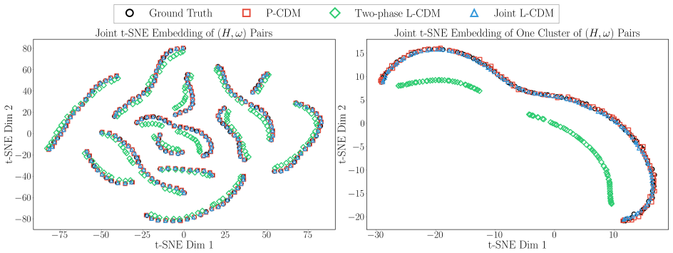
On the paper's own terms, the central discovery is a failure mode and its cure. Latent diffusion models are normally built in two stages: an autoencoder is trained for reconstruction, and a diffusion model is then trained in the resulting latent space. The paper demonstrates on the 2-D Kolmogorov flow that the reconstruction-optimal latent space is hostile to diffusion sampling: the separately trained autoencoder compresses the $64\times 64$ fields to $16\times 16$ latent codes with tiny reconstruction error (relative error 1.4% for the closure field), yet the conditional diffusion model trained in that space generates physical-space closures with relative error 0.29, more than double the 0.13 of the physical-space baseline. When the autoencoder and the diffusion model are optimized together through a loss that combines reconstructing the closure field, denoising score matching, and a KL term that prevents the latent distribution from collapsing, the same diffusion architecture recovers baseline-level accuracy (relative error 0.11) while keeping the latent-space speed advantage. The interpretation is that joint training lets the encoder discover a latent geometry in which the conditional score function $s_\theta(\tau, z_H, z_\omega)$ is easy to learn, and the paper supports this with t-SNE and energy-spectrum comparisons showing that jointly trained samples align with the ground-truth distribution, plus full 20-second vorticity simulations in which the joint closure stays accurate at roughly an order-of-magnitude lower ensemble cost.
Load-bearing premise
Everything rests on the assumption that the missing physics is fully determined by the current resolved flow field, since the closure is drawn from a distribution conditioned only on the instantaneous vorticity, with no dependence on the flow's history or on unobserved variables, so in flows where unresolved dynamics carry long temporal correlations or hidden degrees of freedom the learned distribution would be misspecified and the reported accuracy would not transfer.
Editorial extensions
If this is right
- The measured cost of a 1000-member closure ensemble for the 2-D Kolmogorov flow drops from about 2.64 seconds of pure generation for the physical-space model to about 0.49 seconds for the latent model, and the full ensemble simulation from roughly 8,650 to 1,240 seconds, the ~10x acceleration the paper reports in Section 3.3.
- Because the framework is written for the general partially known system $\partial V/\partial t = \mathcal{M}(V) + \mathcal{U}(V)$ with the closure drawn from $p(H|\omega)$, the same joint-trained latent pipeline applies to other PDE systems with stochastic, non-local unknown terms, not only to the tested vorticity equation.
- Each closure evaluation is a full-field random draw, so a 1000-member ensemble delivers both a mean correction and a spread that serves as a subgrid uncertainty estimate without extra machinery.
- The score network's Fourier neural operator backbone keeps the latent model in the same architectural family as the resolution-invariant physical-space closure of [29], so the latent version inherits the route toward cross-discretization operation that the authors name as future work.
Reading between the lines
- I read the two-phase failure as a geometric effect that likely generalizes beyond closure modeling: reconstruction-optimal encoders can arrange the target distribution so that its conditional score is hard to approximate, so any latent diffusion application with continuous fields as conditioning, such as super-resolution or spatiotemporal forecasting, could exhibit the same gap, and the Table 3 co
- The memoryless assumption is the natural next pressure point: conditioning the sampler on a short history of $\omega$ would reveal how much temporal correlation the subgrid term actually carries, and I expect the gap between memoryless and memory-augmented closures to widen as the Reynolds number grows or forcing becomes more intermittent.
- With the cost barrier lowered, a follow-up the authors do not report becomes feasible: checking whether the 1000-sample spread of generated closures brackets the true error of the resolved simulation across many initial conditions, turning the speedup into a quantitative statement about calibration of the model's uncertainty estimates.
Editorial analysis
A structured set of objections, weighed in public.
Referee Report
Summary. The paper proposes a latent conditional diffusion model (L-CDM) for stochastic closure modeling of nonlinear dynamical systems, focusing on a 2D Kolmogorov flow. A convolutional autoencoder compresses 64x64 resolved-vorticity and closure fields to 16x16 latent representations, and a Fourier-neural-operator-based score model is trained in that latent space. The authors contrast conventional two-phase training (autoencoder first, diffusion second) with a joint training objective that combines reconstruction, score matching, and KL regularization. They report that jointly trained L-CDM matches the generation accuracy of a physical-space conditional diffusion model (P-CDM) while being substantially faster, and they integrate the model into ensemble simulations of the vorticity equation. The paper claims roughly 10x acceleration in ensemble simulation with comparable predictive accuracy.
Significance. If the claims held as stated, the paper would make a useful practical contribution: it demonstrates that latent-space diffusion can serve as a computationally cheaper stochastic closure while preserving accuracy, and it provides evidence that joint training of the autoencoder and score model improves generative fidelity relative to the conventional two-phase pipeline. The internal comparison in Tables 3 and 4 is coherent and the improvement of joint L-CDM over two-phase L-CDM is consistent across generation metrics. The paper also reports detailed architecture and hyperparameter choices. However, the central numerical claim is currently weakened by a direct inconsistency between the closure term defined in Section 3 and the closure term implemented in Appendix A.2, and the reported speedup in Table 5 (6.99x) does not match the repeated '~10x' claim. The absence of code or data, and the use of a single flow regime, further limit verification. The core idea is defensible, but the manuscript needs substantial clarification and revision before the claims can be accepted.
major comments (4)
- [Section 3.3 / Appendix A.2] There is a direct contradiction in what the learned model replaces. Section 3 defines the unknown closure as H(x,t) = -u·∇ω + βξ (Eq. 26) and Table 5 reports errors for this closure. Appendix A.2 states that the ground-truth correction term is G†(x,t) = ν∇²ω + 2βξ, and Eq. (A.7) rewrites the Crank-Nicolson update so that the surrogate model G replaces G†. Since Eq. (A.6) still computes the exact advection F_n = u·∇ω, the simulation may actually be validating a latent model for viscous-plus-stochastic forcing, not for the advection-plus-stochastic term that the paper claims to learn. This changes the difficulty of the learning problem and the meaning of the results. Please clarify which definition was used in the reported experiments, and release the solver code or data so the reader can determine which closure was actually sampled.
- [Section 3.3 / Table 5 / Abstract / Conclusion] The paper repeatedly claims a '~10x acceleration' (abstract, Section 3.3, Conclusion), but Table 5 reports ensemble simulation costs of 1236.87 s for joint L-CDM versus 8652.49 s for P-CDM, which is a factor of 6.99, not 10. In addition, the Introduction's bullet list claims 'orders-of-magnitude faster inference,' yet the generation times in Section 3.1 show only 5.5x acceleration (2.64 s vs. 0.48 s). The reported numbers do not support the stated magnitude of the speedup; please correct the claims or provide a consistent measurement that supports them.
- [Section 2.2.2 / Tables 3 and 4] The improvement of joint L-CDM over two-phase L-CDM is attributed to joint optimization, but the joint objective in Eq. (22) also introduces KL regularization (λ_KL) that is absent from the two-phase baseline. The paper does not provide an ablation that isolates the effect of joint optimization from the effect of latent-space regularization. A two-phase pipeline with a KL-regularized autoencoder would clarify whether the observed gain is due to the joint training itself or simply to preventing latent-space collapse. This distinction is load-bearing for the paper's main methodological claim.
- [Section 3 / Reproducibility] The experimental evidence is confined to one flow regime, and no code or data are provided. Given the closure-definition ambiguity raised above, the absence of an explicit solver specification makes the central result impossible to verify independently. At minimum, the authors should provide the numerical implementation (or a precise pseudocode of the integration loop) and, ideally, a second test case (e.g., different Reynolds number or forcing) to support the general claim of stochastic and non-local closure modeling.
minor comments (6)
- [Eq. (11) and Algorithm 1] The expression for the covariance Σ(τ) is ambiguous: it should read (σ^{2τ} - 1)/(2 ln σ) I, consistent with the perturbation used in Algorithm 1. The current typography '1/2 logσ' can be misread as (1/2) log σ times (σ^{2τ} - 1).
- [Table 5 footnote] The time-cost definitions are not fully clear: the footnote says per-sample cost is the average wall-clock time per trajectory and ensemble cost is the total time to generate and average 1000 samples, but it does not state whether the ensemble simulation runs one trajectory with 1000 samples at each evaluation or 1000 independent trajectories. Please specify explicitly, along with the number of score evaluations per trajectory.
- [Section 3.3] The text states that closure terms are generated every 5 physical timesteps, but it does not state the total number of closure evaluations per 20-second simulation. This number is needed to interpret the reported wall-clock times and to compare per-sample versus ensemble costs.
- [Figure 9 / Eq. (31)] Eq. (31) defines an energy spectrum E(k,t) from the Fourier transform of the closure field H, but Figure 9 shows energy spectra of the resolved vorticity. Please define the spectrum used in Figure 9 explicitly or clarify how Eq. (31) is adapted to the vorticity field.
- [Abstract and Introduction] Minor copyediting: the abstract contains the duplicated phrase 'for many real-world applications', and the phrase 'in physical spaces' should be singular 'in physical space'. The Introduction also states 'prohibitive computational inference cost limits practical applications for many real-world applications', which repeats the same wording.
- [Section 3.2 / Figure 5] The t-SNE caption states that the left panel shows 'Ten distinct clusters corresponding to different test trajectories', but the visual appears to contain more than ten distinguishable clusters. Please clarify how the ten trajectories are represented and how the colors are assigned.
Circularity Check
No significant circularity: the joint latent-diffusion closure is evaluated by out-of-sample rollout, and self-citations to the authors' prior work are not load-bearing.
full rationale
The paper's derivation chain is an empirical training-and-rollout loop rather than a formal reduction: the conditional closure distribution p(H|omega) is learned from paired snapshots, and the central claims in Section 3.3 are tested by integrating the trained models into a numerical solver on held-out trajectories (Table 5 reports per-sample and ensemble-mean errors over 1000 independent simulations). No fitted parameter is renamed as a prediction, and the reported 10x acceleration is a measured wall-clock comparison of the same sampling procedure in latent versus physical space. The only self-citations are to the authors' prior work [29], used to motivate the P-CDM baseline ('we implement a physical-space conditional diffusion model (P-CDM) following the methodology established in [29]') and to reference an adaptive time-stepping scheme and the score-matching equivalence; none of these citations supplies the paper's central conclusion, which rests on the paper's own Tables 3-5. There is an internal inconsistency worth noting as a correctness concern, not as circularity: Section 3 defines the unknown target as H = -u dot grad omega + beta xi, while Appendix A.2 states 'Recall that in Section 3, we have the ground truth of the correction term G-dagger(x,t) = nu Laplacian omega + 2 beta xi' and rewrites the solver update with G-dagger; this ambiguity affects which quantity was actually learned and simulated, but it does not make the empirical comparison circular. No load-bearing uniqueness theorem or ansatz is imported from the authors' prior work, and the numerical results are self-contained comparisons among models trained and evaluated under the same protocol.
Assumptions & free parameters
free parameters (3)
- Loss weights lambda_H, lambda_omega, lambda_score, lambda_KL =
10, 0.1, 0.1, 0.01
- VE SDE scale sigma and final time T =
not reported
- Latent resolution 16x16 =
16x16 (from 64x64 fields)
assumptions (4)
- standard math Equivalence between explicit score matching and denoising score matching (Eq. 13)
- domain assumption The closure term is determined by the instantaneous resolved state V, so p(H|omega) needs no memory
- domain assumption Training data from 20-40 s of 90 trajectories at 64x64 are representative of the target regime
- ad hoc to paper KL regularization on the latent space prevents collapse and preserves diffusion stochasticity
Cite this review
Pith. "Pith review of Stochastic and Non-local Closure Modeling for Nonlinear Dynamical Systems via Latent Score-based Generative Models." pith.science (2026). https://pith.science/paper/2YWNU46M
@misc{pith2026250620771,
  author       = {Pith},
  title        = {Pith review of: Stochastic and Non-local Closure Modeling for Nonlinear Dynamical Systems via Latent Score-based Generative Models},
  year         = {2026},
  howpublished = {\url{https://pith.science/paper/2YWNU46M}},
  note         = {Machine review of arXiv:2506.20771}
}
read the original abstract
We propose a latent score-based generative AI framework for learning stochastic, non-local closure models and constitutive laws in nonlinear dynamical systems of computational mechanics. This work addresses a key challenge of modeling complex multiscale dynamical systems without a clear scale separation, for which numerically resolving all scales is prohibitively expensive, e.g., for engineering turbulent flows. While classical closure modeling methods leverage domain knowledge to approximate subgrid-scale phenomena, their deterministic and local assumptions can be too restrictive in regimes lacking a clear scale separation. Recent developments of diffusion-based stochastic models have shown promise in the context of closure modeling, but their prohibitive computational inference cost limits practical applications in many real-world settings. This work addresses this limitation by jointly training convolutional autoencoders with conditional diffusion models in latent space, significantly reducing the dimensionality of the sampling process while preserving essential physical characteristics. Numerical results demonstrate that the joint training approach helps discover a proper latent space that not only guarantees small reconstruction errors but also ensures good performance of the diffusion model in the latent space. When integrated into numerical simulations, the proposed stochastic modeling framework via latent conditional diffusion models achieves significant computational acceleration while maintaining comparable predictive accuracy to standard diffusion models in physical space.
Figures


Figures from the paper (6 more)



Reference graph
Works this paper leans on
-
[1]
P. Moin, J. Kim, Tackling turbulence with supercomputers, Scientific American 276 (1997) 62–68
1997
-
[2]
P. Moin, K. Mahesh, Direct numerical simulation: A tool in turbulence research, Annual review of fluid mechanics 30 (1998) 539–578
1998
-
[3]
Duraisamy, G
K. Duraisamy, G. Iaccarino, H. Xiao, Turbulence modeling in the age of data, Annual review of fluid mechanics 51 (2019) 357–377
2019
-
[4]
G. A. Holzapfel, Nonlinear solid mechanics: a continuum approach for engineering science, 2002. 23
2002
-
[5]
J. N. Fuhg, G. Anantha Padmanabha, N. Bouklas, B. Bahmani, W. Sun, N. N. Vlassis, M. Flaschel, P. Carrara, L. De Lorenzis, A review on data-driven constitutive laws for solids, Archives of Computational Methods in Engineering (2024) 1–43
2024
-
[6]
Majda, X
A. Majda, X. Wang, Nonlinear dynamics and statistical theories for basic geophysical flows, Cambridge University Press, 2006
2006
-
[7]
Schneider, S
T. Schneider, S. Lan, A. Stuart, J. Teixeira, Earth system modeling 2.0: A blueprint for models that learn from observations and targeted high-resolution simulations, Geo- physical Research Letters 44 (2017) 12–396
2017
-
[8]
J. F. Donges, Y. Zou, N. Marwan, J. Kurths, Complex networks in climate dynamics: Comparinglinearandnonlinearnetworkconstructionmethods, TheEuropeanPhysical Journal Special Topics 174 (2009) 157–179
2009
Show all 103 references
-
[9]
C.-Y. Lai, P. Hassanzadeh, A. Sheshadri, M. Sonnewald, R. Ferrari, V. Balaji, Machine learning for climate physics and simulations, Annual Review of Condensed Matter Physics 16 (2024)
2024
-
[10]
Schneider, L
T. Schneider, L. R. Leung, R. C. Wills, Opinion: Optimizing climate models with process-knowledge, resolution, and AI, EGUsphere 2024 (2024) 1–26
2024
-
[11]
Jost, Dynamical systems: examples of complex behaviour, Springer Science & Busi- ness Media, 2005
J. Jost, Dynamical systems: examples of complex behaviour, Springer Science & Busi- ness Media, 2005
2005
-
[12]
E. M. Izhikevich, Dynamical systems in neuroscience, MIT press, 2007
2007
-
[13]
B. E. Launder, D. B. Spalding, The numerical computation of turbulent flows, in: Numerical prediction of flow, heat transfer, turbulence and combustion, Elsevier, 1983, pp. 96–116
1983
-
[14]
D. C. Wilcox, et al., Turbulence modeling for CFD, volume 2, DCW industries La Canada, CA, 1998
1998
-
[15]
Smagorinsky, General circulation experiments with the primitive equations: I
J. Smagorinsky, General circulation experiments with the primitive equations: I. the basic experiment, Monthly weather review 91 (1963) 99–164
1963
-
[16]
J. W. Deardorff, A numerical study of three-dimensional turbulent channel flow at large Reynolds numbers, Journal of Fluid Mechanics 41 (1970) 453–480
1970
-
[17]
Arnold, Stochastic differential equations: Theory and applications, (No Title) (1974)
L. Arnold, Stochastic differential equations: Theory and applications, (No Title) (1974)
1974
-
[18]
A. Y. Klimenko, R. W. Bilger, Conditional moment closure for turbulent combustion, Progress in energy and combustion science 25 (1999) 595–687
1999
-
[19]
Part I: Model description and testing, Journal of Applied Meteorology and Climatology 46 (2007) 1383–1395
J.E.Pleim, Acombinedlocalandnonlocalclosuremodelfortheatmosphericboundary layer. Part I: Model description and testing, Journal of Applied Meteorology and Climatology 46 (2007) 1383–1395. 24
2007
-
[20]
A. J. Chorin, F. Lu, Discrete approach to stochastic parametrization and dimension reduction in nonlinear dynamics, Proceedings of the National Academy of Sciences 112 (2015) 9804–9809
2015
-
[21]
X.-H. Zhou, J. Han, H. Xiao, Learning nonlocal constitutive models with neural net- works, Computer Methods in Applied Mechanics and Engineering 384 (2021) 113927
2021
-
[22]
Chen, Stochastic methods for modeling and predicting complex dynamical systems, Springer, 2023
N. Chen, Stochastic methods for modeling and predicting complex dynamical systems, Springer, 2023
2023
-
[23]
J.-L. Wu, M. E. Levine, T. Schneider, A. Stuart, Learning about structural errors in models of complex dynamical systems, Journal of Computational Physics 513 (2024) 113157
2024
-
[24]
Chen, J.-L
C. Chen, J.-L. Wu, Neural dynamical operator: Continuous spatial-temporal model with gradient-based and derivative-free optimization methods, Journal of Computa- tional Physics 520 (2025) 113480
2025
-
[25]
J. Sun, Z. Zhang, H. Schaeffer, Lemon: Learning to learn multi-operator networks, arXiv preprint arXiv:2408.16168 (2024)
2024 arXiv
-
[26]
H. You, Y. Yu, S. Silling, M. D’Elia, Nonlocal operator learning for homogenized models: From high-fidelity simulations to constitutive laws, Journal of Peridynamics and Nonlocal Modeling 6 (2024) 709–724
2024
-
[27]
Y. Yu, N. Liu, F. Lu, T. Gao, S. Jafarzadeh, S. A. Silling, Nonlocal attention operator: Materializing hidden knowledge towards interpretable physics discovery, Advances in Neural Information Processing Systems 37 (2024) 113797–113822
2024
-
[28]
X.-H. Zhou, J. Han, M. I. Zafar, E. M. Wolf, C. R. Schrock, C. J. Roy, H. Xiao, Neural operator-based super-fidelity: A warm-start approach for accelerating steady- state simulations, Journal of Computational Physics 529 (2025) 113871
2025
-
[29]
X. Dong, C. Chen, J.-L. Wu, Data-driven stochastic closure modeling via conditional diffusion model and neural operator, Journal of Computational Physics (2025) 114005
2025
-
[30]
Sanderse, P
B. Sanderse, P. Stinis, R. Maulik, S. E. Ahmed, Scientific machine learning for closure models in multiscale problems: A review, 2025. URL:https://www.aimsciences. org/article/id/6705073e8dfec03d48097326. doi:10.3934/fods.2024043
2025
-
[31]
LeCun, Y
Y. LeCun, Y. Bengio, G. Hinton, Deep learning, nature 521 (2015) 436–444
2015
-
[32]
Goodfellow, Y
I. Goodfellow, Y. Bengio, A. Courville, Y. Bengio, Deep learning, volume 1, MIT press Cambridge, 2016
2016
-
[33]
Cristianini, J
N. Cristianini, J. Shawe-Taylor, An introduction to support vector machines and other kernel-based learning methods, Cambridge university press, 2000
2000
-
[34]
L. P. Kaelbling, M. L. Littman, A. W. Moore, Reinforcement learning: A survey, Journal of artificial intelligence research 4 (1996) 237–285. 25
1996
-
[35]
Baker, F
N. Baker, F. Alexander, T. Bremer, A. Hagberg, Y. Kevrekidis, H. Najm, M. Parashar, A. Patra, J. Sethian, S. Wild, et al., Workshop report on basic research needs for sci- entific machine learning: Core technologies for artificial intelligence, Technical Report, USDOE Office o...
2019
-
[36]
K. J. Bergen, P. A. Johnson, M. V. de Hoop, G. C. Beroza, Machine learning for data-driven discovery in solid earth geoscience, Science 363 (2019) eaau0323
2019
-
[37]
Carleo, I
G. Carleo, I. Cirac, K. Cranmer, L. Daudet, M. Schuld, N. Tishby, L. Vogt-Maranto, L. Zdeborová, Machine learning and the physical sciences, Reviews of Modern Physics 91 (2019) 045002
2019
-
[38]
H. Wang, T. Fu, Y. Du, W. Gao, K. Huang, Z. Liu, P. Chandak, S. Liu, P. Van Katwyk, A.Deac, etal., Scientificdiscoveryintheageofartificialintelligence, Nature620(2023) 47–60
2023
-
[39]
Maulik, O
R. Maulik, O. San, A. Rasheed, P. Vedula, Subgrid modelling for two-dimensional turbulence using neural networks, Journal of Fluid Mechanics 858 (2019) 122–144
2019
-
[40]
S. Rasp, M. S. Pritchard, P. Gentine, Deep learning to represent subgrid processes in climate models, Proceedings of the national academy of sciences 115 (2018) 9684–9689
2018
-
[41]
S. H. Rudy, S. L. Brunton, J. L. Proctor, J. N. Kutz, Data-driven discovery of partial differential equations, Science advances 3 (2017) e1602614
2017
-
[42]
Champion, B
K. Champion, B. Lusch, J. N. Kutz, S. L. Brunton, Data-driven discovery of coordi- nates and governing equations, Proceedings of the National Academy of Sciences 116 (2019) 22445–22451
2019
-
[43]
M. L. Gao, J. P. Williams, J. N. Kutz, Sparse identification of nonlinear dynamics and Koopman operators with shallow recurrent decoder networks, arXiv preprint arXiv:2501.13329 (2025)
2025 arXiv
-
[44]
Wang, J.-L
J.-X. Wang, J.-L. Wu, H. Xiao, Physics-informed machine learning approach for recon- structing Reynolds stress modeling discrepancies based on DNS data, Physical Review Fluids 2 (2017) 034603
2017
-
[45]
Karpatne, G
A. Karpatne, G. Atluri, J. H. Faghmous, M. Steinbach, A. Banerjee, A. Ganguly, S. Shekhar, N. Samatova, V. Kumar, Theory-guided data science: A new paradigm for scientific discovery from data, IEEE Transactions on knowledge and data engineering 29 (2017) 2318–2331
2017
-
[46]
J.-L. Wu, H. Xiao, E. Paterson, Physics-informed machine learning approach for augmenting turbulence models: A comprehensive framework, Physical Review Fluids 3 (2018) 074602
2018
-
[47]
Raissi, P
M. Raissi, P. Perdikaris, G. E. Karniadakis, Physics-informed neural networks: A deep learning framework for solving forward and inverse problems involving nonlinear partial differential equations, Journal of Computational physics 378 (2019) 686–707. 26
2019
-
[48]
L. Sun, H. Gao, S. Pan, J.-X. Wang, Surrogate modeling for fluid flows based on physics-constrained deep learning without simulation data, Computer Methods in Applied Mechanics and Engineering 361 (2020) 112732
2020
-
[49]
R. Wang, R. Yu, Physics-guided deep learning for dynamical systems: A survey, arXiv preprint arXiv:2107.01272 (2021)
2021 arXiv
-
[50]
Kashinath, M
K. Kashinath, M. Mustafa, A. Albert, J. Wu, C. Jiang, S. Esmaeilzadeh, K. Aziz- zadenesheli, R. Wang, A. Chattopadhyay, A. Singh, et al., Physics-informed machine learning: Case studies for weather and climate modelling, Philosophical Transactions of the Royal Society A 379 (2...
2021
-
[51]
G. E. Karniadakis, I. G. Kevrekidis, L. Lu, P. Perdikaris, S. Wang, L. Yang, Physics- informed machine learning, Nature Reviews Physics 3 (2021) 422–440
2021
-
[52]
Willard, X
J. Willard, X. Jia, S. Xu, M. Steinbach, V. Kumar, Integrating scientific knowledge with machine learning for engineering and environmental systems, ACM Computing Surveys 55 (2022) 1–37
2022
-
[53]
P. J. Baddoo, B. Herrmann, B. J. McKeon, J. Nathan Kutz, S. L. Brunton, Physics- informed dynamic mode decomposition, Proceedings of the Royal Society A 479 (2023) 20220576
2023
-
[54]
Sharma, W
P. Sharma, W. T. Chung, B. Akoush, M. Ihme, A review of physics-informed machine learning in fluid mechanics, Energies 16 (2023) 2343
2023
-
[55]
R. Yu, R. Wang, Learning dynamical systems from data: An introduction to physics- guided deep learning, Proceedings of the National Academy of Sciences 121 (2024) e2311808121
2024
-
[56]
A. Beck, D. Flad, C.-D. Munz, Deep neural networks for data-driven LES closure models, Journal of Computational Physics 398 (2019) 108910
2019
-
[57]
Rezende, S
D. Rezende, S. Mohamed, Variational inference with normalizing flows, in: Interna- tional conference on machine learning, PMLR, 2015, pp. 1530–1538
2015
-
[58]
J. Ho, A. Jain, P. Abbeel, Denoising diffusion probabilistic models, Advances in neural information processing systems 33 (2020) 6840–6851
2020
-
[59]
Y. Song, S. Ermon, Generative modeling by estimating gradients of the data distribu- tion, Advances in neural information processing systems 32 (2019)
2019
-
[60]
Y. Song, J. Sohl-Dickstein, D. P. Kingma, A. Kumar, S. Ermon, B. Poole, Score- based generative modeling through stochastic differential equations, arXiv preprint arXiv:2011.13456 (2020)
2020 arXiv
-
[61]
Rombach, A
R. Rombach, A. Blattmann, D. Lorenz, P. Esser, B. Ommer, High-resolution image synthesis with latent diffusion models, in: Proceedings of the IEEE/CVF conference on computer vision and pattern recognition, 2022, pp. 10684–10695. 27
2022
-
[62]
Z. Kong, W. Ping, J. Huang, K. Zhao, B. Catanzaro, Diffwave: A versatile diffusion model for audio synthesis, arXiv preprint arXiv:2009.09761 (2020)
2020 arXiv
-
[63]
Saharia, W
C. Saharia, W. Chan, S. Saxena, L. Li, J. Whang, E. L. Denton, K. Ghasemipour, R. Gontijo Lopes, B. Karagol Ayan, T. Salimans, et al., Photorealistic text-to-image diffusion models with deep language understanding, Advances in neural information processing systems 35 (2022) 36...
2022
-
[64]
Dhariwal, A
P. Dhariwal, A. Nichol, Diffusion models beat GANs on image synthesis, Advances in neural information processing systems 34 (2021) 8780–8794
2021
-
[65]
A. Q. Nichol, P. Dhariwal, Improved denoising diffusion probabilistic models, in: International conference on machine learning, PMLR, 2021, pp. 8162–8171
2021
-
[66]
Stinis, T
P. Stinis, T. Hagge, A. M. Tartakovsky, E. Yeung, Enforcing constraints for interpola- tion and extrapolation in generative adversarial networks, Journal of Computational Physics 397 (2019) 108844
2019
-
[67]
D. J. Gagne, H. M. Christensen, A. C. Subramanian, A. H. Monahan, Machine learn- ing for stochastic parameterization: Generative adversarial networks in the Lorenz’96 model, Journal of Advances in Modeling Earth Systems 12 (2020) e2019MS001896
2020
-
[68]
L. Yang, D. Zhang, G. E. Karniadakis, Physics-informed generative adversarial net- works for stochastic differential equations, SIAM Journal on Scientific Computing 42 (2020) A292–A317
2020
-
[69]
J.-L. Wu, K. Kashinath, A. Albert, D. Chirila, H. Xiao, et al., Enforcing statistical constraints in generative adversarial networks for modeling chaotic dynamical systems, Journal of Computational Physics 406 (2020) 109209
2020
-
[70]
Stinis, C
P. Stinis, C. Daskalakis, P. J. Atzberger, Sdyn-gans: Adversarial learning methods for multistep generative models for general order stochastic dynamics, Journal of Computational Physics 519 (2024) 113442
2024
-
[71]
X. Fan, D. Akhare, J.-X. Wang, Neural differentiable modeling with diffusion-based super-resolution for two-dimensional spatiotemporal turbulence, Computer Methods in Applied Mechanics and Engineering 433 (2025) 117478
2025
-
[72]
M. Xu, L. Yu, Y. Song, C. Shi, S. Ermon, J. Tang, Geodiff: A geometric diffusion model for molecular conformation generation, arXiv preprint arXiv:2203.02923 (2022)
2022 arXiv
-
[73]
Y. Song, L. Shen, L. Xing, S. Ermon, Solving inverse problems in medical imaging with score-based generative models, arXiv preprint arXiv:2111.08005 (2021)
2021 arXiv
-
[74]
L. Li, R. Carver, I. Lopez-Gomez, F. Sha, J. Anderson, Generative emulation of weather forecast ensembles with diffusion models, Science Advances 10 (2024) eadk4489. 28
2024
-
[75]
X.-Y. Liu, M. H. Parikh, X. Fan, P. Du, Q. Wang, Y.-F. Chen, J.-X. Wang, Confild- inlet: Synthetic turbulence inflow using generative latent diffusion models with neural fields, arXiv preprint arXiv:2411.14378 (2024)
2024 arXiv
-
[76]
T. Li, A. S. Lanotte, M. Buzzicotti, F. Bonaccorso, L. Biferale, Multi-scale recon- struction of turbulent rotating flows with generative diffusion models, Atmosphere 15 (2023) 60
2023
-
[77]
D. Shu, Z. Li, A. B. Farimani, A physics-informed diffusion model for high-fidelity flow field reconstruction, Journal of Computational Physics 478 (2023) 111972
2023
-
[78]
H. Wen, Y. Lin, Y. Xia, H. Wan, Q. Wen, R. Zimmermann, Y. Liang, Diffstg: Proba- bilistic spatio-temporal graph forecasting with denoising diffusion models, in: Proceed- ings of the 31st ACM International Conference on Advances in Geographic Information Systems, 2023, pp. 1–12
2023
-
[79]
Rasul, C
K. Rasul, C. Seward, I. Schuster, R. Vollgraf, Autoregressive denoising diffusion models for multivariate probabilistic time series forecasting, in: International conference on machine learning, PMLR, 2021, pp. 8857–8868
2021
-
[80]
Tashiro, J
Y. Tashiro, J. Song, Y. Song, S. Ermon, Csdi: Conditional score-based diffusion models for probabilistic time series imputation, Advances in neural information processing systems 34 (2021) 24804–24816
2021
-
[81]
Zhuang, S
Y. Zhuang, S. Cheng, K. Duraisamy, Spatially-aware diffusion models with cross- attention for global field reconstruction with sparse observations, Computer Methods in Applied Mechanics and Engineering 435 (2025) 117623
2025
-
[82]
Jacobsen, Y
C. Jacobsen, Y. Zhuang, K. Duraisamy, Cocogen: Physically consistent and condi- tioned score-based generative models for forward and inverse problems, SIAM Journal on Scientific Computing 47 (2025) C399–C425
2025
-
[83]
Z. Li, N. Kovachki, K. Azizzadenesheli, B. Liu, K. Bhattacharya, A. Stuart, A. Anand- kumar, Fourier neural operator for parametric partial differential equations, arXiv preprint arXiv:2010.08895 (2020)
2020 arXiv
-
[84]
C. Lu, Y. Zhou, F. Bao, J. Chen, C. Li, J. Zhu, Dpm-solver: A fast ode solver for diffusion probabilistic model sampling in around 10 steps, Advances in Neural Information Processing Systems 35 (2022) 5775–5787
2022
-
[85]
L. Liu, Y. Ren, Z. Lin, Z. Zhao, Pseudo numerical methods for diffusion models on manifolds, arXiv preprint arXiv:2202.09778 (2022)
2022 arXiv
-
[86]
Y. Song, P. Dhariwal, M. Chen, I. Sutskever, Consistency models, in: Proceedings of the 40th International Conference on Machine Learning, ICML’23, JMLR.org, 2023
2023
-
[87]
Salimans, J
T. Salimans, J. Ho, Progressive distillation for fast sampling of diffusion models, in: International Conference on Learning Representations, 2022. 29
2022
-
[88]
Luhman, T
E. Luhman, T. Luhman, Knowledge distillation in iterative generative models for improved sampling speed, arXiv preprint arXiv:2101.02388 (2021)
2021 arXiv
-
[89]
Karras, M
T. Karras, M. Aittala, T. Aila, S. Laine, Elucidating the design space of diffusion- basedgenerativemodels, AdvancesinNeuralInformationProcessingSystems35(2022) 26565–26577
2022
-
[90]
Z. Kong, W. Ping, On fast sampling of diffusion probabilistic models, arXiv preprint arXiv:2106.00132 (2021)
2021 arXiv
-
[91]
Vahdat, K
A. Vahdat, K. Kreis, J. Kautz, Score-based generative modeling in latent space, Ad- vances in neural information processing systems 34 (2021) 11287–11302
2021
-
[92]
Esser, R
P. Esser, R. Rombach, B. Ommer, Taming transformers for high-resolution image syn- thesis, in: Proceedings of the IEEE/CVF conference on computer vision and pattern recognition, 2021, pp. 12873–12883
2021
-
[93]
Kingma, T
D. Kingma, T. Salimans, B. Poole, J. Ho, Variational diffusion models, Advances in neural information processing systems 34 (2021) 21696–21707
2021
-
[94]
Vincent, A connection between score matching and denoising autoencoders, Neural Computation 23 (2011) 1661–1674
P. Vincent, A connection between score matching and denoising autoencoders, Neural Computation 23 (2011) 1661–1674
2011
-
[95]
H. Liu, Z. Chen, Y. Yuan, X. Mei, X. Liu, D. Mandic, W. Wang, M. D. Plumbley, Audioldm: Text-to-Audio generation with latent diffusion models, in: International Conference on Machine Learning, PMLR, 2023, pp. 21450–21474
2023
-
[96]
Takagi, S
Y. Takagi, S. Nishimoto, High-resolution image reconstruction with latent diffusion models from human brain activity, in: Proceedings of the IEEE/CVF Conference on Computer Vision and Pattern Recognition, 2023, pp. 14453–14463
2023
-
[97]
Podell, Z
D. Podell, Z. English, K. Lacey, A. Blattmann, T. Dockhorn, J. Müller, J. Penna, R. Rombach, SDXL: Improving latent diffusion models for high-resolution image syn- thesis, in: The Twelfth International Conference on Learning Representations, 2024. URL:https://openreview.net/fo...
2024
-
[98]
Y. Li, Y. Cheng, M. van der Schaar, A study of posterior stability for time-series latent diffusion, arXiv preprint arXiv:2405.14021 (2024)
2024 arXiv
-
[99]
Nguyen, C.-H
B. Nguyen, C.-H. Lai, Y. Takida, N. Murata, T. Uesaka, S. Ermon, Y. Mitsufuji, Im- proving vector-quantized image modeling with latent consistency-matching diffusion, in: ICLR 2025 Workshop on Deep Generative Model in Machine Learning: Theory, Principle and Efficacy, 2025. URL...
2025
-
[100]
Dieleman, L
S. Dieleman, L. Sartran, A. Roshannai, N. Savinov, Y. Ganin, P. H. Richemond, A. Doucet, R. Strudel, C. Dyer, C. Durkan, et al., Continuous diffusion for categorical data, arXiv preprint arXiv:2211.15089 (2022). 30
2022 arXiv
-
[101]
4664–4683
Z.Gao, J.Guo, X.Tan, Y.Zhu, F.Zhang, J.Bian, L.Xu, Empoweringdiffusionmodels on the embedding space for text generation, in: NAACL-HLT, 2024, pp. 4664–4683. URL:https://doi.org/10.18653/v1/2024.naacl-long.261
2024 doi
-
[102]
Vahdat, J
A. Vahdat, J. Kautz, Nvae: A deep hierarchical variational autoencoder, Advances in neural information processing systems 33 (2020) 19667–19679
2020
-
[103]
Tancik, P
M. Tancik, P. Srinivasan, B. Mildenhall, S. Fridovich-Keil, N. Raghavan, U. Singhal, R. Ramamoorthi, J. Barron, R. Ng, Fourier features let networks learn high frequency functions in low dimensional domains, Advances in neural information processing systems 33 (2020) 7537–7547...
2020
Reviewed August 6, 2026 · model on record in the stance chip above.
Discussion (0). Sign in to comment.