REVIEW 3 major objections 4 minor 1 cited by
The Wasserstein normalized autoencoder replaces the usual reconstruction-only loss with a Wasserstein distance between data and model distribution, and this single change lets an autoencoder trained only on background jets flag exotic jets
Reviewed by Pith at T0; open to challenge. T0 means a machine referee read the full paper against a public rubric. the ladder, T0–T4 →
T0 review · deepseek-v4-flash
2026-08-04 12:42 UTC pith:33UQCEO3
load-bearing objection The WNAE is a genuinely new training objective that fixes a real AE failure mode, but the headline claim of full signal-agnosticism is weakened by signal-dependent MCMC tuning in Appendix C. the 3 major comments →
Wasserstein normalized autoencoder for anomaly detection
The pith
A machine-rendered reading of the paper's core claim, the machinery that carries it, and where it could break.
Core claim
The central claim is that minimizing the Wasserstein distance W(p_data, p_theta) between the empirical training distribution and the Boltzmann distribution p_theta(x) proportional to exp(−E_theta(x)), with E_theta the mean-squared reconstruction error of the autoencoder, trains the network to learn the probability density of the inlier data instead of merely reconstructing it. As a result, outliers—points with low density under the training distribution—receive high reconstruction error and are separated from background. Concretely, a network trained on background jets reaches AUC 0.69–0.77 for semivisible-jet signals across a grid of mediator masses and invisible fractions, while a plain au
What carries the argument
The load-bearing object is the Wasserstein distance W(p_data, p_theta), computed on minibatches: the positive samples are training (background) examples, and the negative samples are drawn from p_theta by a Langevin Monte Carlo chain, initialized with persistent contrastive divergence and run for ten steps. Because the negative samples depend on the network weights through the gradient of the energy, the implementation retains the computational graph through the chain so gradients of the Wasserstein distance flow back into the autoencoder. The energy is the autoencoder's mean-squared reconstruction error, so the same network is both the feature extractor and the energy model. A key differenc
Load-bearing premise
Everything rests on the assumption that ten Langevin Monte Carlo steps, seeded by persistent contrastive divergence, produce samples close enough to the model's Boltzmann distribution that the minibatch Wasserstein distance between those negative samples and the training data is a faithful estimate of W(p_data, p_theta); if the chain is too short, the loss being minimized is not the stated Wasserstein distance and the training and stopping logic no longer follow.
What would settle it
Train the same WNAE on a low-dimensional synthetic mixture where the exact Wasserstein distance can be computed numerically, then compare the training loss (minibatch Wasserstein with 10 MCMC steps) to the exact distance. If the two diverge systematically as training proceeds, or if increasing the chain length to 100 changes the learned AUC by more than a few percent on the semivisible-jet task, the claim that the objective is the Wasserstein distance is falsified.
If this is right
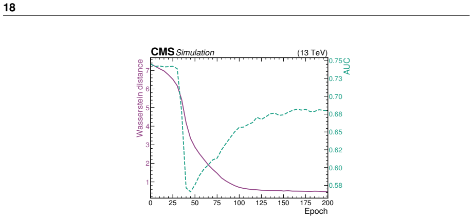
- If the central claim holds, autoencoder-based anomaly detection no longer needs a separate validation signal to detect overtraining: the minimum of the validation Wasserstein distance is the recommended stopping point, and it matches peak discrimination.
- The approach remains fully unsupervised; the signal is never used during training, yet performance is stable across a range of signal hypotheses, which supports its use as a model-agnostic search tool.
- The WNAE mitigates complexity bias: when trained on semivisible-jet signal events, it tags ordinary top-jets as anomalous, whereas a plain autoencoder fails in that reversed setup.
- Training is stable and convergent without ad-hoc regularization, because the Wasserstein objective does not reward the unbounded growth of the negative energy that plagues the earlier normalized autoencoder.
Where Pith is reading between the lines
- Editorial inference: The same signal-agnostic Wasserstein distance could be used as an early-stopping or quality metric for other generative models and energy-based methods, not only autoencoders.
- Editorial inference: A natural stress test outside the paper is to fix the number of Langevin steps at a larger value, such as 100, and check whether the learned AUC and the validation Wasserstein minimum remain unchanged; if they move, the effective objective is a contrastive-divergence approximation rather than the true Wasserstein distance.
- Editorial inference: The paper's iterative self-supervised refinement idea, retraining on low-reconstruction-error examples, could turn WNAE into a tool for weakly supervised searches where the training sample is contaminated by unknown anomalies.
Editorial analysis
A structured set of objections, weighed in public.
Referee Report
Summary. The paper introduces the Wasserstein normalized autoencoder (WNAE), an autoencoder-based anomaly detection method in which the reconstruction error defines a Boltzmann energy, and training minimizes the Wasserstein distance between the data distribution and the model distribution, with the model distribution sampled by Langevin MCMC. The method is applied to separating semivisible jets from a ttbar background in CMS simulation. The authors report that a standard autoencoder yields AUC ≈ 0.5 due to outlier reconstruction, that the normalized autoencoder (NAE) suffers from training instability and mode collapse, and that the WNAE trains stably, has a signal-agnostic stopping criterion based on the Wasserstein distance, and achieves AUCs around 0.69–0.77 across a grid of SVJ signal hypotheses, while also mitigating complexity bias.
Significance. If the claims are fully supported, the WNAE would be a practically useful anomaly detection method for jet substructure, with two concrete strengths: it addresses a known failure mode of autoencoders (outlier reconstruction) and it ships with public source code and detailed appendices on the gradient propagation and learning-rate schedule. The central empirical result—stable WNAE training with a Wasserstein-based stopping criterion—is plausible and interesting. However, the strongest advertised property, full signal-agnosticism, is weakened by the signal-dependent selection of MCMC hyperparameters in Appendix C. This issue is fixable, but it currently prevents the paper from establishing the headline claim as stated.
major comments (3)
- [Appendix C, Table C.1; Section 4.4, Fig. 11] The MCMC hyperparameters (λ = 0.0242, σ = 0.22, T = 0.063, restart fraction r = 0.05) are explicitly optimized to maximize the AUC for discrimination between SVJs and top-quark jets, using Eq. (20) as the loss function. The same family of SVJ signal models is then used to report the WNAE AUC grid in Fig. 11. The abstract's claim that the WNAE 'remains fully agnostic to the signal' is therefore not supported by the presented evidence: the model configuration was selected using signal labels. The two added constraints (matching negative/positive feature distributions and minimizing the Wasserstein distance) mitigate but do not eliminate this dependence; they do not certify performance on a different, unseen signal. Please either (a) select MCMC hyperparameters using only background-derived criteria before evaluating any signal hypothesis, or (b) present a nested evaluation in which the sig
- [Section 2.4, Appendix C, Section 4.1, Fig. 10] The negative samples that approximate p_theta are produced with only 10 Langevin steps per batch, using persistent contrastive divergence. No convergence diagnostics, autocorrelation estimates, or sensitivity scans in N_MCMC are shown. If the chain has not converged, the quantity minimized in Eq. (21) is not W(p_data, p_theta), and the interpretation of the Wasserstein-distance curves and the kink-based stopping condition loses its stated meaning. Tuning the MCMC hyperparameters on signal AUC (Appendix C) cannot substitute for a demonstration that the sampler is faithful. Please add a convergence check (for example, comparing negative-sample feature distributions with validation data over training, reporting sensitivity to N_MCMC, or estimating effective sample sizes), or explicitly state that the loss is an approximation to the Wasserstein distance whose reliability is assessed only ind
- [Section 4.4, Fig. 11] The AUC grid is reported without statistical uncertainties. Since the test background set is 15% of 47k jets and the signal samples are model-dependent, differences between neighboring grid points (e.g., 0.745 vs. 0.749) may not be significant. Please provide bootstrap or other uncertainties, and state which training epoch/stopping criterion was used to produce Fig. 11, so the reader can verify that the minimum validation Wasserstein distance is indeed the reported point.
minor comments (4)
- [Eq. (16), Section 2.5] The notation F_L is used for the set of 1-Lipschitz functions but is never defined. Please define it explicitly, for example as {f: |f(x)−f(y)| ≤ ||x−y||}.
- [Appendix C, Table C.1] The text says the hyperparameters are optimized using Eq. (20), which is the NAE log-cosh loss. Since the WNAE uses a different loss, please state explicitly whether the same hyperparameters are reused for the WNAE training in Section 4.3, or whether they were re-tuned. This is important for reproducibility.
- [Fig. 10] The left panel legend contains 'Signal vs. Background' and 'Signal vs. Negative' curves. Since the training is claimed to be unsupervised, the caption should clarify that signal samples are overlaid only for illustration and are not used in the loss or stopping criterion.
- [Reference [65]] The source code repository is referenced without a version, DOI, or commit identifier. Please add a persistent identifier or version number to support reproducibility.
Circularity Check
MCMC hyperparameters are tuned on SVJ-vs-top AUC, so the reported WNAE AUC grid is partly a selected result rather than an independent signal-agnostic prediction.
specific steps
-
fitted input called prediction
[Appendix C, 'Tuning the MCMC' (discussion preceding Table C.1)]
"These parameters are optimized to maximize the AUC for discrimination between SVJs and top quark jets, using Eq. (20) as the loss function, with two constraints to mitigate bias toward the signal hypothesis."
The WNAE's headline performance, Fig. 11, reports AUC on a grid of SVJ signal models, while Appendix C says the MCMC hyperparameters (T, sigma, lambda, r) were themselves optimized to maximize the AUC for discrimination between SVJs and top-quark jets. Thus the reported AUCs are not an out-of-sample, signal-agnostic evaluation: the configuration was selected using the same signal class and the same metric that are then presented as the result. The two constraints (matching positive/negative feature distributions and minimizing the Wasserstein distance) mitigate but do not remove the dependence, because the final choice among configurations satisfying those constraints was still made by maximizing SVJ-vs-top AUC. Consequently, Fig. 11 is partly a report of the selection criterion, not an in
full rationale
The core WNAE derivation is mathematically self-contained: the Boltzmann-form p_theta with energy equal to reconstruction error, the MLE gradient expressed through MCMC negative samples, and the replacement of the NAE energy-difference loss by the minibatch Wasserstein distance between positive and negative samples are all well-defined and do not reduce to their inputs by construction. There is no load-bearing self-citation or imported uniqueness theorem. The central circularity concern is confined to the empirical evaluation: Appendix C explicitly tunes MCMC hyperparameters to maximize the same SVJ-vs-top AUC that is later reported in Fig. 11 as evidence of 'strong classification performance... while remaining fully agnostic to the signal.' Because the hyperparameters were selected using signal labels and the target metric, the reported AUCs carry an optimistic selection bias and do not by themselves establish the advertised signal-agnostic property. The paper's own warning—that AUC-optimal configurations with mismatched negative/positive distributions would 'bias the performance... towards the signal hypotheses used for tuning'—shows the selection mechanism is real, even though the two constraints were intended to guard against the most extreme bias. This is a partial circularity in the evaluation claim, not in the algorithm's derivation, so the score is 6 rather than higher.
Axiom & Free-Parameter Ledger
free parameters (6)
- MCMC step size λ =
0.0242
- MCMC noise coefficient σ =
0.22
- Langevin temperature T =
0.063
- Number of MCMC steps =
10
- MCMC restart fraction =
0.05
- NAE Wasserstein-kink stopping threshold =
not specified
axioms (6)
- ad hoc to paper Reconstruction error defines a Boltzmann energy: pθ(x) ∝ exp(−lθ(x)) (Eqs. 1–3).
- domain assumption Langevin MCMC with σ=√(2λ) converges to pθ in the infinite-step limit (Eq. 13), and 10 steps are sufficient in practice.
- domain assumption Minimizing W(p_data, pθ) yields an energy function that orders points by data density, so low-density anomalies receive high reconstruction error.
- domain assumption The 8 chosen jet-substructure features (major/minor axes, EFP1, C2(0.5), pT^D, soft-drop mass, τ2, τ3) suffice to separate SVJ signal from ttbar background.
- domain assumption Simulated ttbar and SVJ samples faithfully represent LHC data and dark-sector signals.
- standard math Minibatch Wasserstein distance provides unbiased gradient estimates.
read the original abstract
A novel anomaly detection algorithm is presented. The Wasserstein normalized autoencoder (WNAE) is a normalized probabilistic model that minimizes the Wasserstein distance between the learned probability distribution--a Boltzmann distribution where the energy is the reconstruction error of the autoencoder--and the distribution of the training data. This algorithm has been developed and applied to the identification of semivisible jets--conical sprays of visible standard model particles and invisible dark matter states--with the CMS experiment at the CERN LHC. Trained on jets of particles from simulated standard model processes, the WNAE is shown to learn the probability distribution of the input data in a fully unsupervised fashion, such that it effectively identifies new physics jets as anomalies. The model exhibits stable, convergent training and recovers strong classification performance for a wide range of signals against the selected background process, for which a standard autoencoder fails because of outlier reconstruction. In addition, the model improves upon standard normalized autoencoders while remaining fully agnostic to the signal. The WNAE directly tackles the problem of outlier reconstruction, a common failure mode of autoencoders in anomaly detection tasks.
Figures


Forward citations
Cited by 1 Pith paper
-
Machine-learning techniques for model-independent searches in dijet final states
Five ML anomaly-detection methods enhance model-agnostic dijet searches at CMS, and a weakly supervised tagger identifies hadronic top-quark decays in data nearly as well as a supervised classifier.
Reference graph
Works this paper leans on
-
[1]
T. Heimel, G. Kasieczka, T. Plehn, and J. M. Thompson, “QCD or what?”,SciPost Phys.6 (2019) 030,doi:10.21468/SciPostPhys.6.3.030,arXiv:1808.08979. 20
Pith/arXiv arXiv 2019
-
[2]
Searching for new physics with deep autoencoders
M. Farina, Y. Nakai, and D. Shih, “Searching for new physics with deep autoencoders”, Phys. Rev. D101(2020) 075021,doi:10.1103/PhysRevD.101.075021, arXiv:1808.08992
Pith/arXiv arXiv 2020
-
[3]
Autoencoders for unsupervised anomaly detection in high energy physics
T. Finke et al., “Autoencoders for unsupervised anomaly detection in high energy physics”,JHEP06(2021) 161,doi:10.1007/JHEP06(2021)161, arXiv:2104.09051
Pith/arXiv arXiv 2021
-
[4]
Autoencoding under normalization constraints
S. Yoon, Y.-K. Noh, and F. Park, “Autoencoding under normalization constraints”, in Proceedings of the 38th International Conference on Machine Learning, p. 12087. 2021. arXiv:2105.05735
Pith/arXiv arXiv 2021
-
[5]
Semivisible jets: Dark matter undercover at the LHC
T. Cohen, M. Lisanti, and H. K. Lou, “Semivisible jets: Dark matter undercover at the LHC”,Phys. Rev. Lett.115(2015) 171804,doi:10.1103/PhysRevLett.115.171804, arXiv:1503.00009
Pith/arXiv arXiv 2015
-
[6]
The CMS experiment at the CERN LHC
CMS Collaboration, “The CMS experiment at the CERN LHC”,JINST3(2008) S08004, doi:10.1088/1748-0221/3/08/S08004
-
[7]
Development of the CMS detector for the CERN LHC Run 3
CMS Collaboration, “Development of the CMS detector for the CERN LHC Run 3”, JINST19(2024) P05064,doi:10.1088/1748-0221/19/05/P05064, arXiv:2309.05466
Pith/arXiv arXiv 2024
-
[8]
Performance of the CMS Level-1 trigger in proton-proton collisions at √s=13 TeV
CMS Collaboration, “Performance of the CMS Level-1 trigger in proton-proton collisions at √s=13 TeV”,JINST15(2020) P10017, doi:10.1088/1748-0221/15/10/P10017,arXiv:2006.10165
Pith/arXiv arXiv 2020
-
[9]
CMS Collaboration, “The CMS trigger system”,JINST12(2017) P01020, doi:10.1088/1748-0221/12/01/P01020,arXiv:1609.02366
Pith/arXiv arXiv 2017
-
[10]
Performance of the CMS high-level trigger during LHC run 2
CMS Collaboration, “Performance of the CMS high-level trigger during LHC run 2”, JINST19(2024) P11021,doi:10.1088/1748-0221/19/11/P11021, arXiv:2410.17038
Pith/arXiv arXiv 2024
-
[11]
Electron and photon reconstruction and identification with the CMS experiment at the CERN LHC
CMS Collaboration, “Electron and photon reconstruction and identification with the CMS experiment at the CERN LHC”,JINST16(2021) P05014, doi:10.1088/1748-0221/16/05/P05014,arXiv:2012.06888
Pith/arXiv arXiv 2021
-
[12]
CMS Collaboration, “Performance of the CMS muon detector and muon reconstruction with proton-proton collisions at √s=13 TeV”,JINST13(2018) P06015, doi:10.1088/1748-0221/13/06/P06015,arXiv:1804.04528
Pith/arXiv arXiv 2018
-
[13]
Description and performance of track and primary-vertex reconstruction with the CMS tracker
CMS Collaboration, “Description and performance of track and primary-vertex reconstruction with the CMS tracker”,JINST9(2014) P10009, doi:10.1088/1748-0221/9/10/P10009,arXiv:1405.6569
Pith/arXiv arXiv 2014
-
[14]
Particle-flow reconstruction and global event description with the CMS detector
CMS Collaboration, “Particle-flow reconstruction and global event description with the CMS detector”,JINST12(2017) P10003,doi:10.1088/1748-0221/12/10/P10003, arXiv:1706.04965
Pith/arXiv arXiv 2017
-
[15]
Jet energy scale and resolution in the CMS experiment in pp collisions at 8 TeV
CMS Collaboration, “Jet energy scale and resolution in the CMS experiment in pp collisions at 8 TeV”,JINST12(2017) P02014, doi:10.1088/1748-0221/12/02/P02014,arXiv:1607.03663. References 21
Pith/arXiv arXiv 2017
-
[16]
CMS Collaboration, “Performance of missing transverse momentum reconstruction in proton-proton collisions at √s=13 TeV using the CMS detector”,JINST14(2019) P07004,doi:10.1088/1748-0221/14/07/P07004,arXiv:1903.06078
Pith/arXiv arXiv 2019
-
[17]
Mathematical methods of organizing and planning production
L. V . Kantorovich, “Mathematical methods of organizing and planning production”, Management Science6(1939) 366,doi:10.1287/mnsc.6.4.366
-
[18]
Markov processes over denumerable products of spaces describing large systems of automata
L. N. Vaserstein, “Markov processes over denumerable products of spaces describing large systems of automata”,Problems of Information Transmission5(1969) 47
1969
-
[19]
Autoassociative neural networks
M. A. Kramer, “Autoassociative neural networks”,Comput. Chem. Eng.16(1992) 313, doi:10.1016/0098-1354(92)80051-A
-
[20]
P . Smolensky, “Parallel Distributed Processing, Volume 1: Explorations in the Microstructure of Cognition: Foundations”, ch. Information processing in dynamical systems: Foundations of harmony theory. The MIT Press, 1986. doi:10.7551/mitpress/5236.003.0009
-
[21]
Training products of experts by minimizing contrastive divergence
G. Hinton, “Training products of experts by minimizing contrastive divergence”,Neural Comput.14(2002) 1771,doi:10.1162/089976602760128018
-
[22]
Energy-based models for sparse overcomplete representations
Y. W. Teh, M. Welling, S. Osindero, and G. E. Hinton, “Energy-based models for sparse overcomplete representations”,J. Mach. Learn. Res.4(2003) 1235
2003
-
[23]
Information theory and statistical mechanics
E. T. Jaynes, “Information theory and statistical mechanics”,Phys. Rev.106(1957) 620, doi:10.1103/PhysRev.106.620
-
[24]
Auto-encoding variational Bayes
D. P . Kingma and M. Welling, “Auto-encoding variational Bayes”, in2nd International Conference on Learning Representations. 2014.arXiv:1312.6114
Pith/arXiv arXiv 2014
-
[25]
A. Makhzani, J. Shlens, N. Jaitly, and I. Goodfellow, “Adversarial autoencoders”, in International Conference on Learning Representations. 2016.arXiv:1511.05644
Pith/arXiv arXiv 2016
-
[26]
I. J. Goodfellow et al., “Generative adversarial nets”, inAdvances in Neural Information Processing Systems, volume 27, p. 2672. Curran Associates, Inc., 2014. arXiv:1406.2661
Pith/arXiv arXiv 2014
-
[27]
I. Tolstikhin, O. Bousquet, S. Gelly, and B. Schoelkopf, “Wasserstein auto-encoders”, in International Conference on Learning Representations. 2018.arXiv:1711.01558
Pith/arXiv arXiv 2018
-
[28]
On a space of totally additive functions
L. V . Kantorovich and S. Rubinshtein, “On a space of totally additive functions”,Vestnik of the St. Petersburg University: Mathematics13(1958) 52
1958
-
[29]
M. Arjovsky, S. Chintala, and L. Bottou, “Wasserstein GAN”, inProceedings of the 34th International Conference on Machine Learning, volume 70, p. 214. 2017. arXiv:1701.07875
Pith/arXiv arXiv 2017
-
[30]
POT: Python optimal transport
R. Flamary et al., “POT: Python optimal transport”,J. Mach. Learn. Res.22(2021) 1
2021
-
[31]
Learning with minibatch Wasserstein: asymptotic and gradient properties
K. Fatras et al., “Learning with minibatch Wasserstein: asymptotic and gradient properties”, inProceedings of the Twenty Third International Conference on Artificial Intelligence and Statistics, volume 108, p. 2131. 2019.arXiv:1910.04091
Pith/arXiv arXiv 2019
-
[32]
Do deep generative models know what they don’t know?
E. Nalisnick et al., “Do deep generative models know what they don’t know?”, in International Conference on Learning Representations. 2019.arXiv:1810.09136. 22
Pith/arXiv arXiv 2019
-
[33]
Likelihood regret: An out-of-distribution detection score for variational auto-encoder
Z. Xiao, Q. Yan, and Y. Amit, “Likelihood regret: An out-of-distribution detection score for variational auto-encoder”, inAdvances in Neural Information Processing Systems, volume 33, p. 20685. 2020.arXiv:2003.02977
Pith/arXiv arXiv 2020
-
[34]
Generative probabilistic novelty detection with adversarial autoencoders
S. Pidhorskyi, R. Almohsen, and G. Doretto, “Generative probabilistic novelty detection with adversarial autoencoders”, inProceedings of the 32nd International Conference on Neural Information Processing Systems, p. 6823. 2018.arXiv:1807.02588
Pith/arXiv arXiv 2018
-
[35]
GANomaly: Semi-supervised anomaly detection via adversarial training
S. Akcay, A. Atapour-Abarghouei, and T. P . Breckon, “GANomaly: Semi-supervised anomaly detection via adversarial training”, inAsian Conference on Computer Vision, p. 622, Springer. 2018.arXiv:1805.06725. doi:10.1007/978-3-030-20893-6_39
Pith/arXiv arXiv 2018
-
[36]
f-AnoGAN: Fast unsupervised anomaly detection with generative adversarial networks
T. Schlegl et al., “f-AnoGAN: Fast unsupervised anomaly detection with generative adversarial networks”,Medical Image Analysis54(2019) 30, doi:10.1016/j.media.2019.01.010
-
[37]
Implicit generation and modeling with energy-based models
Y. Du and I. Mordatch, “Implicit generation and modeling with energy-based models”, in Proceedings of the 33rd International Conference on Neural Information Processing Systems, p. 324. 2019.arXiv:1903.08689
Pith/arXiv arXiv 2019
-
[38]
Realtime anomaly detection at the L1 trigger of CMS experiment
A. Gandrakota, “Realtime anomaly detection at the L1 trigger of CMS experiment”,PoS ICHEP2024(2025) 1025,doi:10.22323/1.476.1025,arXiv:2411.19506
Pith/arXiv arXiv 2025
-
[39]
CMS Collaboration, “Model-agnostic search for dijet resonances with anomalous jet substructure in proton-proton collisions at √s= 13 TeV”,Rept. Prog. Phys.88(2025) 067802,doi:10.1088/1361-6633/add762,arXiv:2412.03747
Pith/arXiv arXiv 2025
-
[40]
ATLAS Collaboration, “Search for new phenomena in two-body invariant mass distributions using unsupervised machine learning for anomaly detection at √s=13 TeV with the ATLAS detector”,Phys. Rev. Lett.132(2024) 081801, doi:10.1103/PhysRevLett.132.081801,arXiv:2307.01612
Pith/arXiv arXiv 2024
-
[41]
A normalized autoencoder for LHC triggers
B. M. Dillon et al., “A normalized autoencoder for LHC triggers”,SciPost Phys. Core6 (2023) 074,doi:10.21468/SciPostPhysCore.6.4.074,arXiv:2206.14225
arXiv 2023
-
[42]
V . C. Rubin, N. Thonnard, and W. K. Ford, Jr., “Rotational properties of 21 SC galaxies with a large range of luminosities and radii, from NGC 4605 (R = 4 kpc) to UGC 2885 (R = 122 kpc)”,Astrophys. J.238(1980) 471,doi:10.1086/158003
doi:10.1086/158003 1980
-
[43]
The universal rotation curve of spiral galaxies: I. The dark matter connection
M. Persic, P . Salucci, and F. Stel, “The universal rotation curve of spiral galaxies: I. The dark matter connection”,Mon. Not. Roy. Astron. Soc.281(1996) 27, doi:10.1093/mnras/278.1.27,arXiv:astro-ph/9506004
Pith/arXiv arXiv 1996
-
[44]
A direct empirical proof of the existence of dark matter
D. Clowe et al., “A direct empirical proof of the existence of dark matter”,Astrophys. J. 648(2006) L109,doi:10.1086/508162,arXiv:astro-ph/0608407
Pith/arXiv arXiv 2006
-
[45]
Dark Energy Survey year 1 results: curved-sky weak lensing mass map
DES Collaboration, “Dark Energy Survey year 1 results: curved-sky weak lensing mass map”,Mon. Not. Roy. Astron. Soc.475(2018) 3165,doi:10.1093/mnras/stx3363, arXiv:1708.01535
Pith/arXiv arXiv 2018
-
[46]
Planck 2018 results. VI. Cosmological parameters
Planck Collaboration, “Planck 2018 results. VI. Cosmological parameters”,Astron. Astrophys.641(2020) A6,doi:10.1051/0004-6361/201833910, arXiv:1807.06209. [Erratum:doi:10.1051/0004-6361/201833910e]. References 23
Pith/arXiv arXiv 2018
-
[47]
Echoes of a hidden valley at hadron colliders
M. J. Strassler and K. M. Zurek, “Echoes of a hidden valley at hadron colliders”,Phys. Lett. B651(2007) 374,doi:10.1016/j.physletb.2007.06.055, arXiv:hep-ph/0604261
Pith/arXiv arXiv 2007
-
[48]
Search for resonant production of strongly coupled dark matter in proton-proton collisions at 13 TeV
CMS Collaboration, “Search for resonant production of strongly coupled dark matter in proton-proton collisions at 13 TeV”,JHEP06(2022) 156, doi:10.1007/JHEP06(2022)156,arXiv:2112.11125
Pith/arXiv arXiv 2022
-
[49]
ATLAS Collaboration, “Search for new physics in final states with semivisible jets or anomalous signatures using the ATLAS detector”,Phys. Rev. D112(2025) 012021, doi:10.1103/44zp-mh1q,arXiv:2505.01634
Pith/arXiv arXiv 2025
-
[50]
LHC searches for dark sector showers
T. Cohen, M. Lisanti, H. K. Lou, and S. Mishra-Sharma, “LHC searches for dark sector showers”,JHEP11(2017) 196,doi:10.1007/JHEP11(2017)196, arXiv:1707.05326
Pith/arXiv arXiv 2017
-
[51]
Strongly interacting dark sectors in the early universe and at the LHC through a simplified portal
E. Bernreuther, F. Kahlhoefer, M. Kr¨amer, and P . Tunney, “Strongly interacting dark sectors in the early universe and at the LHC through a simplified portal”,JHEP01 (2020) 162,doi:10.1007/JHEP01(2020)162,arXiv:1907.04346
Pith/arXiv arXiv 2020
-
[52]
J. Alwall et al., “The automated computation of tree-level and next-to-leading order differential cross sections, and their matching to parton shower simulations”,JHEP07 (2014) 079,doi:10.1007/JHEP07(2014)079,arXiv:1405.0301
Pith/arXiv arXiv 2014
-
[53]
T. Sj ¨ostrand et al., “An introduction to PYTHIA 8.2”,Comput. Phys. Commun.191(2015) 159,doi:10.1016/j.cpc.2015.01.024,arXiv:1410.3012
Pith/arXiv arXiv 2015
-
[54]
GEANT4 Collaboration, “GEANT4—a simulation toolkit”,Nucl. Instrum. Meth. A506 (2003) 250,doi:10.1016/S0168-9002(03)01368-8
-
[55]
Parton distributions from high-precision collider data
NNPDF Collaboration, “Parton distributions from high-precision collider data”,Eur. Phys. J. C77(2017) 663,doi:10.1140/epjc/s10052-017-5199-5, arXiv:1706.00428
Pith/arXiv arXiv 2017
-
[56]
The anti-kT jet clustering algorithm
M. Cacciari, G. P . Salam, and G. Soyez, “The anti-kT jet clustering algorithm”,JHEP04 (2008) 063,doi:10.1088/1126-6708/2008/04/063,arXiv:0802.1189
Pith/arXiv arXiv 2008
-
[57]
M. Cacciari, G. P . Salam, and G. Soyez, “FastJet user manual”,Eur. Phys. J. C72(2012) 1896,doi:10.1140/epjc/s10052-012-1896-2,arXiv:1111.6097
Pith/arXiv arXiv 2012
-
[58]
Performance of quark/gluon discrimination in 8 TeV pp data
CMS Collaboration, “Performance of quark/gluon discrimination in 8 TeV pp data”, CMS Physics Analysis Summary CMS-PAS-JME-13-002, 2013
2013
-
[59]
Energy flow polynomials: A complete linear basis for jet substructure
P . T. Komiske, E. M. Metodiev, and J. Thaler, “Energy flow polynomials: A complete linear basis for jet substructure”,JHEP04(2018) 013, doi:10.1007/JHEP04(2018)013,arXiv:1712.07124
Pith/arXiv arXiv 2018
-
[60]
Energy correlation functions for jet substructure
A. J. Larkoski, G. P . Salam, and J. Thaler, “Energy correlation functions for jet substructure”,JHEP06(2013) 108,doi:10.1007/JHEP06(2013)108, arXiv:1305.0007
Pith/arXiv arXiv 2013
-
[61]
A. J. Larkoski, S. Marzani, G. Soyez, and J. Thaler, “Soft drop”,JHEP05(2014) 146, doi:10.1007/JHEP05(2014)146,arXiv:1402.2657. 24
Pith/arXiv arXiv 2014
-
[62]
Identifying boosted objects with N-subjettiness
J. Thaler and K. Van Tilburg, “Identifying boosted objects with N-subjettiness”,JHEP03 (2011) 015,doi:10.1007/JHEP03(2011)015,arXiv:1011.2268
Pith/arXiv arXiv 2011
-
[63]
Scikit-learn: Machine learning in Python
F. Pedregosa et al., “Scikit-learn: Machine learning in Python”,J. Mach. Learn. Res.12 (2011) 2825,arXiv:1201.0490
Pith/arXiv arXiv 2011
-
[64]
Autoencoders for semivisible jet detection
F. Canelli et al., “Autoencoders for semivisible jet detection”,JHEP02(2022) 074, doi:10.1007/JHEP02(2022)074,arXiv:2112.02864
Pith/arXiv arXiv 2022
-
[65]
https://gitlab.cern.ch/cms-analysis/mlg/mlg-24-002/wnae
Source code repository, 2025. https://gitlab.cern.ch/cms-analysis/mlg/mlg-24-002/wnae
2025
-
[66]
PyTorch: An imperative style, high-performance deep learning library
A. Paszke et al., “PyTorch: An imperative style, high-performance deep learning library”, inProceedings of the 33rd International Conference on Neural Information Processing Systems, volume 32, p. 721. 2019.arXiv:1912.01703
Pith/arXiv arXiv 2019
-
[67]
Training restricted Boltzmann machines using approximations to the likelihood gradient
T. Tieleman, “Training restricted Boltzmann machines using approximations to the likelihood gradient”, inProceedings of the 25th International Conference on Machine Learning, p. 1064. 2008.doi:10.1145/1390156.1390290. A Gradient dependence between MCMC and AE During the MCMC process, the gradient with respect to the feature space needs to be calcu- lated ...
arXiv 2008
discussion (0)
Sign in with ORCID, Apple, or X to comment. Anyone can read and Pith papers without signing in.