REVIEW 3 major objections 4 minor 33 references
On the Renormalization Group flow of distributions
T0 review · 3 major / 4 minor · reviewed 2026-08-07 · deepseek-v4-flash
Pith's one-line read The whole distribution, not single trajectories, determines the most probable couplings under RG flow.
desk verdict The mode-vs-trajectory point is correct and useful, Application 1 is solid, but the hypercharge peak in Application 2 is a coordinate artifact and the structure claims are prior-dependent. read the letter →
The pith
A machine-rendered reading of the paper's core claim, the machinery that carries it, and where it could break.
The reading
What carries the argument
The central object is the continuity (Liouville) equation for the probability density on coupling space, $\partial_t P = -\sum_i \partial_{g_i}(\beta_{g_i}P)$, together with its formal solution by the method of characteristics, $P(\vec g,t)=P_0(\vec g_0(t,\vec g))\,\exp[-\int_{t_0}^t dt'\,\sum_i \partial_{g_i}\beta_{g_i}]$. The exponential factor, the Jacobian determinant of the RG flow map, carries all the behavior beyond individual trajectories: it shifts the location of maxima, makes highest-density regions differ from evolved $\sigma$-bands, and makes the distribution asymmetric so that mean and mode do not coincide. For the one-loop hypercharge $\beta$ function $\beta_\alpha=\beta_1\alpha^2$ the paper solves the maximum position in closed form, $\alpha_{\max}(t)$, and shows explicitly that it overshoots and then approaches the infrared-attractive fixed point from the other side rather than being monotonically attracted to it. For the full Standard Model, the same machinery is evaluated numerically by Monte-Carlo sampling of the initial distribution and individual evolution of the samples.
What would settle it
Repeat the application-2 Monte-Carlo evolution with Gaussian widths $\sigma\in\{0.3,1,3\}$ (or with a flat prior on a bounded region) and record the infrared peak locations for $g_Y$ and $\lambda$; if those peaks move by more than about 50 percent from the reported values or vanish, the claim that the flow favours the observed Standard Model values is an artifact of the chosen prior rather than of the flow itself.
Extended reading notes
Core claim
The central claim is that the renormalization-group flow of a probability distribution over couplings is governed by the continuity equation $\partial_t P = -\sum_i \partial_{g_i}(\beta_{g_i}P)$, whose method-of-characteristics solution is $P(\vec g,t)=P_0(\vec g_0(t,\vec g))\,\exp[-\int_{t_0}^{t} dt'\,\sum_i \partial_{g_i}\beta_{g_i}]$. The exponential factor is the Jacobian of the map from initial to final couplings, and it is what invalidates trajectory-by-trajectory reasoning: the stationarity condition $\partial_g P=0$ does not reduce to $\partial_{g_0}P_0=0$ whenever this factor depends on the final couplings. The authors demonstrate the effect analytically for the hypercharge $\beta$ function $\beta_\alpha=\beta_1\alpha^2$, where the maximum of the distribution evolves non-monotonically and approaches the infrared-attractive fixed point $\alpha=0$ only in the infinite-scale limit. The same mechanism, acting through the scale-dependent quasi-fixed point of the Higgs quartic coupling, produces the peaked infrared distributions reported for the Standard Model. As a second demonstration, the most probable value of the Higgs metastability scale is $2.6\times10^{10}$ GeV, which differs from the RG-evolved central value by about a factor of three, and the evolved $\sigma$-intervals are not the highest-density regions of the evolved distribution.
Load-bearing premise
The load-bearing premise is that a unit-width isotropic Gaussian centered at zero is the 'generic' Planck-scale prior for the Standard Model couplings, together with the assumption that trajectories ending in Landau poles may be discarded; changing the prior width or shape, or keeping the divergent trajectories, shifts or removes the emergent peaks.
Editorial extensions
If this is right
- Error propagation in any quantum field theory with uncertain couplings must be performed by evolving the full distribution; evolving only the central value gives wrong maxima, means, and confidence regions.
- The most probable scale of new physics associated with Higgs metastability is $2.6\times10^{10}$ GeV, about a factor of three below the usual RG-evolved central-value estimate.
- Infrared-attractive fixed points do not attract the maximum of the distribution during finite RG time; the maximum can overshoot the fixed point and approach it from the other side.
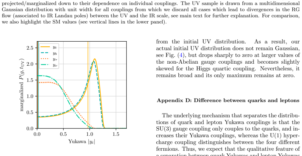
- Starting from a broad, generic Planck-scale distribution, the Standard Model flow produces peaked hypercharge and Higgs quartic distributions near their observed values and reproduces the qualitative third-generation Yukawa ordering.
- The formalism supplies the basis for Bayesian assessment of beyond-Standard-Model settings and of ultraviolet completions whose initial conditions are not unique.
Reading between the lines
- Beyond the paper: the non-monotonic maximum mechanism should be generic in any theory with nonlinear beta functions, so the Standard Model example is likely one instance of a broader distributional phenomenon; this could be tested in toy models with analytically known beta functions.
- Beyond the paper: the reported proximity of the $g_Y$ and $\lambda$ peaks to observed values depends on the prior, and the paper's own footnote 2 notes that adjusting the Gaussian width shifts the hypercharge peak; a systematic scan over prior widths and shapes would show whether the proximity is robust or a consequence of the unit-width choice.
- Beyond the paper: discarding trajectories that hit Landau poles reshapes the effective initial distribution, making it non-Gaussian and slightly skewed in $\lambda$; the emergent peaks are therefore a property of the perturbative subset of trajectories, not of the full Gaussian sample.
- Beyond the paper: read as a likelihood propagator, the distributional evolution equation would allow computing posterior probabilities for individual Standard Model parameters from a Planck-scale prior, turning the reported qualitative proximity into quantitative model comparison.
Editorial analysis
A structured set of objections, weighed in public.
Referee Report
Summary. The paper derives a continuity equation for the RG evolution of a probability distribution on the space of couplings, Eq. (1), and gives the formal solution Eq. (2) in terms of the inverse flow map and a Jacobian factor. The authors argue that the mode and highest-density regions of the evolved distribution cannot be obtained by evolving individual central values, and they demonstrate this in Application 1 by computing the most probable SM Higgs metastability scale. In Application 2 they evolve a unit-width isotropic Gaussian at the Planck scale to the electroweak scale and report that the marginalized IR distributions develop nonzero peaks for the hypercharge and Higgs quartic couplings, that the Yukawa sector shows the qualitative ordering y_t > y_b > y_tau > y_nu, and that the hypercharge and Higgs peaks lie close to observed values.
Significance. The formal result of the paper, that the RG flow of a distribution is governed by a continuity equation whose Jacobian factor can move the mode away from the image of the initial mode, is correct and is a useful cautionary point for error propagation and Bayesian analyses in QFT. Application 1 is a concrete, state-of-the-art demonstration of this effect in the SM Higgs sector. However, the stronger structure-emergence claims in Application 2 are not robust: the reported hypercharge peak is a property of the chosen coordinate and prior, and the prior-width sensitivity is acknowledged in the manuscript itself. The paper is therefore a worthwhile contribution to the methodology, but its headline claims about explaining SM couplings require substantial reframing and additional analysis.
major comments (3)
- [Application 2, Eqs. (5)-(8), Fig. 2] The hypercharge peak at g_Y ≈ 0.5 is not a coordinate-invariant property of the evolved distribution. With the paper's own variable α = g_Y^2/(4π), a UV Gaussian in g_Y induces P_{α0}(α0) ∝ α0^{-1/2} e^{-2π α0}, and applying Eq. (8) gives P_α(α,t) ~ α^{-1/2} as α → 0 for any finite RG time, so the mode remains at α = 0. Thus the 'striking' proximity of the hypercharge peak to the observed value, emphasized in the abstract, is an artifact of the flat measure dg and disappears under a standard reparameterization. The paper does not justify why dg, rather than dα or another measure, is the physically relevant measure on coupling space.
- [Application 2, footnote 2 and Appendix C] The structure-emergence claims depend on a hand-chosen prior: an isotropic unit-width Gaussian centered at zero. Footnote 2 explicitly concedes that adjusting the width moves the peaks toward or away from the observed values, and Appendix C shows that removing Landau-pole trajectories further deforms the initial distribution away from a Gaussian. Without a sensitivity analysis over a reasonable class of priors, the statement that SM-like structures are 'likely' or 'generic' is not supported. This is load-bearing because the abstract's proximity claim for the hypercharge and Higgs quartic couplings rests on this particular prior choice.
- [Application 2, Eq. (9) and Fig. 2] The analytic illustration in Eq. (9) uses an initial Gaussian in α, P0(α) = (1/√(2π)σ) e^{-α^2/(2σ^2)}, which is a different prior from the numerical experiment, which samples an isotropic Gaussian in g. The analytic example therefore does not explain the numerical hypercharge peak in Fig. 2. The numerical peak is instead generated by the Jacobian factors associated with the g-coordinate, as discussed in the first major comment. This inconsistency should be clarified, and the analytic example should be explicitly labeled as a toy model rather than as an explanation of the SM result.
minor comments (4)
- [Eq. (4)] The notation g = (g_Y, g_2, g_3|..., y_t, y_b, y_tau, lambda) with a vertical bar is unusual and unclear; a standard vector notation or a sentence explaining the grouping would improve readability.
- [Fig. 2 caption and main text] The caption refers to a 'lower panel' for the Higgs quartic coupling, but Fig. 2 has three panels; the relevant panel is the right panel.
- [Appendix C and main text] The main text says the initial distribution is a unit-width Gaussian, but Appendix C explains that after excluding Landau-pole trajectories the actual sampled distribution is no longer Gaussian. This conditioning should be stated prominently in the main text, since it affects the interpretation of all subsequent results.
- [Introduction and Application 2] The statement that 'IR-attractive fixed points do not necessarily attract the maximum of the distribution' should be qualified as being coordinate- and prior-dependent, since the mode of a probability density is not invariant under nonlinear reparameterizations.
Circularity Check
Hypercharge 'peak near observed value' is a coordinate artifact: in the standard coupling α=g_Y^2/(4π) the evolved mode stays at the IR fixed point, so the headline proximity claim reduces to the chosen measure and prior width by construction.
-
self definitional
[Application 2, Eqs. (5)–(8), Fig. 2 and footnote 2]
"We work with α= g_Y^2/(4π) and consider β_α=β_1 α^2 ... For the beta-function Eq. (5) and the relation (7) between the initial condition α_0 and the final value α(t), P(α(t),t) in Eq. (2) becomes P(α(t),t)=P_0(α_0(t,α))·(α_0/α)^2. ... A better match with experimental results can be obtained by slightly adjusting the width (or shape) of the initial distribution."
The headline claim that the most probable hypercharge value lies near g_Y≈0.5 is the mode of the density in the coordinate g. Under the paper's actual UV prior, an isotropic unit-width Gaussian in g, the induced prior in α=g_Y^2/(4π) is P_α0(α0) ∝ α0^{-1/2} e^{-2π α0}. Inserting this into the paper's own Eq. (8) gives P_α(α,t) ~ α^{-1/2} as α→0 for every finite RG time t0−t, so the mode in α sits at the IR fixed point α=0. Thus the peak at g_Y≈0.5 is generated by the Jacobian of the coordinate choice, not by the RG flow. Footnote 2 concedes that adjusting the width or shape of the initial distribution changes the match to observations, confirming that the proximity claim is a function of the input prior and coordinate rather than an independent prediction.
full rationale
The core evolution equation (1) and its formal solution (2) are derived from the definition of expectation values and the method of characteristics, with no circular step. Application 1, the metastability-scale calculation, is a direct propagation of the stated top-mass Gaussian through the SM beta functions and is likewise non-circular: the conclusion that the maximum of the distribution is not the RG-evolved central value follows from Eq. (3), not from any fitted parameter. However, Application 2's headline hypercharge result is not parameter-free. With the paper's own UV Gaussian in g_Y, transforming to the standard coupling α=g_Y^2/(4π) makes the evolved density diverge at α=0, so the most probable value in that coordinate remains the IR fixed point; the reported peak at g_Y≈0.5 is an artifact of the chosen coordinate and prior width, as footnote 2 effectively admits. The Yukawa-ordering and Higgs quasi-fixed-point discussions have independent content, and the self-citations [30,31] appear only in the outlook and are not load-bearing. Because one of the two 'striking' proximity claims reduces to the input measure by construction, the paper is partially circular, scoring 6.
Assumptions & free parameters
free parameters (1)
- Initial UV distribution width and mean for SM couplings =
sigma = 1, mu = 0
assumptions (4)
- domain assumption Standard Model beta functions at one-loop (Application 2) and three-loop/two-loop (Application 1) describe the true RG flow over the relevant scales.
- ad hoc to paper The RG flow map g(t, g0) is invertible on the support of the evolved distribution; divergent trajectories are removed to enforce this.
- ad hoc to paper An isotropic unit-width Gaussian centered at zero is a representative 'generic' UV distribution.
- standard math Method of characteristics and the Liouville/continuity equation for probability densities under deterministic flows.
Cite this review
Pith. "Pith review of On the Renormalization Group flow of distributions." pith.science (2026). https://pith.science/paper/3CCY3GKX
@misc{pith2026250612548,
  author       = {Pith},
  title        = {Pith review of: On the Renormalization Group flow of distributions},
  year         = {2026},
  howpublished = {\url{https://pith.science/paper/3CCY3GKX}},
  note         = {Machine review of arXiv:2506.12548}
}
read the original abstract
Renormalization Group flows relate the values of couplings at different scales. Here, we go beyond the Renormalization Group flow of individual trajectories and derive an evolution equation for a distribution on the space of couplings. This shift in perspective can provide new insights, even in theories for which the Renormalization Group flow of individual couplings is well understood. As a first application, we propagate errors under the Renormalization Group flow. Characteristic properties of an error distribution, such as its maximum or highest density region, cannot be propagated at the level of individual couplings, but require our evolution equation for the distribution on the space of couplings. We demonstrate this by calculating the most probable value for the metastability scale in the Higgs sector of the Standard Model. Our second application is the emergence of structure in sets of couplings. We discover that infrared-attractive fixed points do not necessarily attract the maximum of the distribution when the Renormalization Group is evolved over a finite range of scales. Instead, sharply peaked maxima can build up at coupling values that cannot be inferred from individual trajectories. We demonstrate this emergence of structure for the Standard Model, starting from a broad distribution at the Planck scale. The Renormalization Group flow favors the phenomenological ordering of third-generation Yukawa couplings and, strikingly, we find that the most probable values for the Abelian hypercharge and Higgs quartic coupling lie close to their observed values.
Figures


Figures from the paper (2 more)

Reference graph
Works this paper leans on
-
[1]
The second factor, the exponential of the integrated derivative of the beta function, introduces additional nonlinearities into the RG evolution ofP(g, t). It is cru- cial for the maxima of the evolved distribution, because 0 =∂ gP(g, t) = (∂g0 P(g 0))∂ gg0(t, g)·e h − R t t0 dt′ ∂gβg i +P 0(g0(t, g))·∂g e h − R t t0 dt′ ∂gβg i .(3) Requiring∂ g0 P(g 0) =...
arXiv 2025
-
[2]
F. Bezrukov, M. Y. Kalmykov, B. A. Kniehl, and M. Sha- poshnikov, JHEP10, 140 (2012), arXiv:1205.2893 [hep- ph]
arXiv 2012
-
[3]
G. Degrassi, S. Di Vita, J. Elias-Miro, J. R. Espinosa, G. F. Giudice, G. Isidori, and A. Strumia, JHEP08, 098 (2012), arXiv:1205.6497 [hep-ph]
arXiv 2012
-
[4]
P. Q. Hung, Phys. Rev. Lett.42, 873 (1979)
work page 1979
-
[5]
H. D. Politzer and S. Wolfram, Phys. Lett. B82, 242 (1979), [Erratum: Phys.Lett.B 83, 421 (1979)]
1979
- [6]
- [7]
-
[8]
P. B. Arnold, Phys. Rev. D40, 613 (1989)
work page 1989
Show all 33 references
-
[9]
C. Ford, D. R. T. Jones, P. W. Stephenson, and M. B. Einhorn, Nucl. Phys. B395, 17 (1993), arXiv:hep- lat/9210033
1993
-
[10]
Sher, Phys
M. Sher, Phys. Lett. B317, 159 (1993), [Adden- dum: Phys.Lett.B 331, 448–448 (1994)], arXiv:hep- ph/9307342
1993
-
[11]
Altarelli and G
G. Altarelli and G. Isidori, Phys. Lett. B337, 141 (1994)
1994
-
[12]
J. A. Casas, J. R. Espinosa, and M. Quiros, Phys. Lett. B342, 171 (1995), arXiv:hep-ph/9409458
1995 arXiv
-
[13]
J. R. Espinosa and M. Quiros, Phys. Lett. B353, 257 (1995), arXiv:hep-ph/9504241
1995 arXiv
-
[14]
Isidori, G
G. Isidori, G. Ridolfi, and A. Strumia, Nucl. Phys. B 609, 387 (2001), arXiv:hep-ph/0104016
2001 arXiv
-
[15]
Ellis, J
J. Ellis, J. R. Espinosa, G. F. Giudice, A. Hoecker, and A. Riotto, Phys. Lett. B679, 369 (2009), arXiv:0906.0954 [hep-ph]
2009 arXiv
-
[16]
Buttazzo, G
D. Buttazzo, G. Degrassi, P. P. Giardino, G. F. Giudice, F. Sala, A. Salvio, and A. Strumia, JHEP12, 089 (2013), arXiv:1307.3536 [hep-ph]
2013 arXiv
- [17]
-
[18]
Elias-Miro, J
J. Elias-Miro, J. R. Espinosa, G. F. Giudice, H. M. Lee, and A. Strumia, JHEP06, 031 (2012), arXiv:1203.0237 [hep-ph]
2012 arXiv
-
[19]
W. Chao, M. Gonderinger, and M. J. Ramsey-Musolf, Phys. Rev. D86, 113017 (2012), arXiv:1210.0491 [hep- ph]
2012 arXiv
-
[20]
Gabrielli, M
E. Gabrielli, M. Heikinheimo, K. Kannike, A. Racioppi, M. Raidal, and C. Spethmann, Phys. Rev. D89, 015017 (2014), arXiv:1309.6632 [hep-ph]
2014 arXiv
-
[21]
Gies and R
H. Gies and R. Sondenheimer, Eur. Phys. J. C75, 68 (2015), arXiv:1407.8124 [hep-ph]
2015 arXiv
-
[22]
Eichhorn, H
A. Eichhorn, H. Gies, J. Jaeckel, T. Plehn, M. M. Scherer, and R. Sondenheimer, JHEP04, 022 (2015), arXiv:1501.02812 [hep-ph]
2015 arXiv
-
[23]
Ballesteros, J
G. Ballesteros, J. Redondo, A. Ringwald, and C. Tamarit, JCAP08, 001 (2017), arXiv:1610.01639 [hep-ph]
2017 arXiv
-
[24]
Elias-Miro, J
J. Elias-Miro, J. R. Espinosa, G. F. Giudice, G. Isidori, A. Riotto, and A. Strumia, Phys. Lett. B709, 222 (2012), arXiv:1112.3022 [hep-ph]
2012 arXiv
-
[25]
Hiller, T
G. Hiller, T. H¨ ohne, D. F. Litim, and T. Steudtner, Phys. Rev. D110, 115017 (2024), arXiv:2401.08811 [hep-ph]
2024
-
[26]
Navaset al.(Particle Data Group), Phys
S. Navaset al.(Particle Data Group), Phys. Rev. D110, 030001 (2024)
2024
-
[27]
Cvetic, J
M. Cvetic, J. Halverson, G. Shiu, and W. Taylor, (2022), arXiv:2204.01742 [hep-th]
2022 arXiv
-
[28]
Marchesano, G
F. Marchesano, G. Shiu, and T. Weigand, Ann. Rev. Nucl. Part. Sci.74, 113 (2024), arXiv:2401.01939 [hep- th]
2024 arXiv
-
[29]
Constantin, C
A. Constantin, C. S. Fraser-Taliente, T. R. Harvey, A. Lukas, and B. Ovrut, Nucl. Phys. B1010, 116778 (2025), arXiv:2402.01615 [hep-th]
2025 arXiv
-
[30]
Constantin, C
A. Constantin, C. S. Fraser-Taliente, T. R. Harvey, L. T. Y. Leung, and A. Lukas, (2024), arXiv:2410.17704 [hep-th]
2024 arXiv
-
[31]
Eichhorn and A
A. Eichhorn and A. Held, Phys. Lett. B777, 217 (2018), arXiv:1707.01107 [hep-th]
2018 arXiv
-
[32]
Eichhorn and A
A. Eichhorn and A. Held, Phys. Rev. Lett.121, 151302 (2018), arXiv:1803.04027 [hep-th]
2018 arXiv
-
[33]
Eichhorn and M
A. Eichhorn and M. Schiffer, (2022), arXiv:2212.07456 [hep-th]. 6 SUPPLEMENTARY MATERIAL Appendix A: Derivation of the evolution equation for the probability distribution The evolution equation can be derived as follows: We consider an arbitrary functionu(g i) of the couplings...
2022 arXiv
Reviewed August 7, 2026 · model on record in the stance chip above.
Discussion (0). Sign in to comment.