REVIEW 4 major objections 6 minor 47 references
Precise Radial Velocities of Cool Low Mass Stars With iSHELL
T0 review · 4 major / 6 minor · reviewed 2026-08-14 · deepseek-v4-flash
Pith's one-line read A K-band spectrograph with a methane-isotopologue gas cell and a 48-parameter forward model achieves 3–5 m/s radial velocities on cool K and M dwarfs, enough to confirm TESS planet candidates with semi-amplitudes above about 3 m/s.
desk verdict First iSHELL K-band RV precision paper: solid pipeline work, honest limitations, but the m/s claims are internal scatter and need an external check before I'd trust them for TESS follow-up. read the letter →
The pith
A machine-rendered reading of the paper's core claim, the machinery that carries it, and where it could break.
The reading
What carries the argument
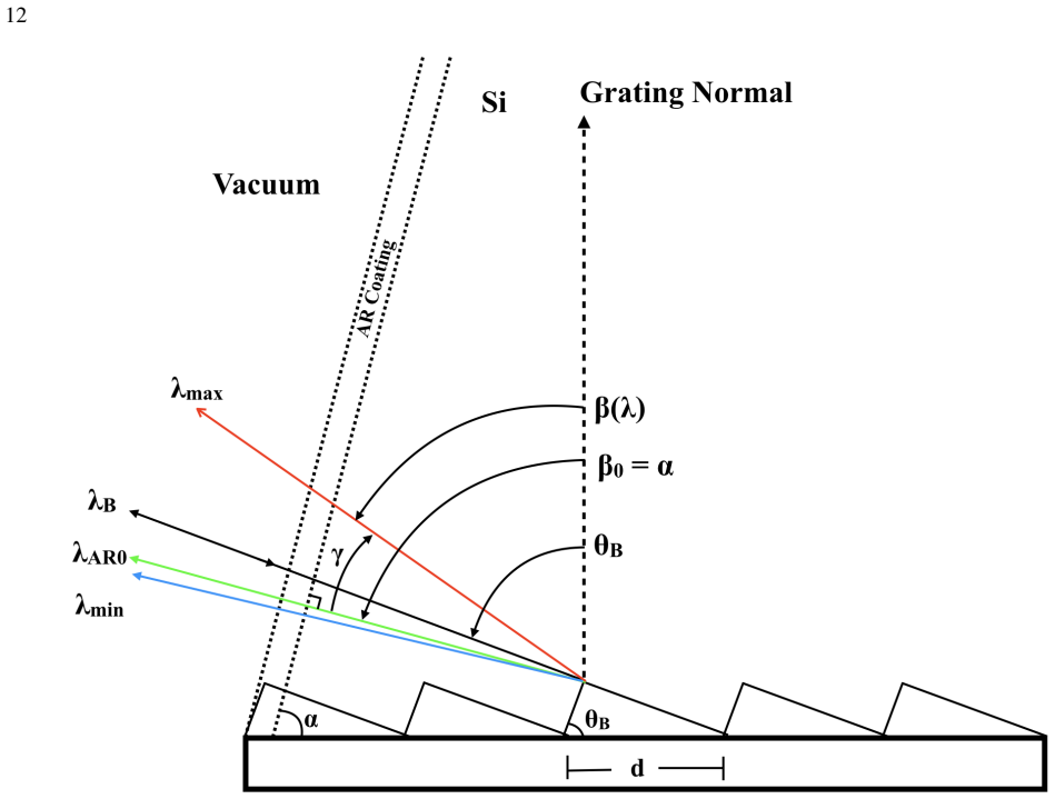
The load-bearing mechanism is the iterative stellar template retrieval: starting from a flat guess, the pipeline forward-models each spectrum, subtracts the model, shifts the residuals into the star's barycentric rest frame, median-combines them with inverse-RMS-squared weights, and adds the result back into the template; after 5–40 iterations the extracted velocities stabilize and the template approaches the deconvolved stellar spectrum. Two calibration devices carry the precision: the methane isotopologue ($^{13}$CH$_4$) gas cell, whose FTS-measured transmission provides a common optical-path wavelength reference and constrains the line-spread function, and explicit Fabry-Perot models for the two fringing sources, the order-selection filter and the anti-reflection coating of the silicon immersion grating. The 48-parameter model is optimized with a custom Nelder-Mead solver that alternates full simplex calls with two-dimensional subspace calls, because standard simplex optimization did not converge in this parameter space.
What would settle it
Inject a known synthetic Doppler shift, for example 10 m/s, into one night's raw spectra before running the pipeline; if the recovered shift differs from the injected value by more than the quoted nightly uncertainty, the stellar template has absorbed correlated noise rather than the true stellar spectrum.
Extended reading notes
Core claim
On its own terms, the paper demonstrates that a 48-parameter forward model can reproduce K-band (2.18–2.47 µm) spectra of cool dwarfs well enough to extract relative radial velocities at the few-m/s level on baselines from one month to one year. The model accounts for the Doppler-shifted stellar spectrum, the methane gas cell transmission, Doppler-shifted telluric water, methane, nitrous oxide, and carbon dioxide, the residual blaze function, a quadratic-plus-spline wavelength solution, the spectrograph line-spread function, and two separate quasi-sinusoidal fringing patterns from the order-selection filter and the immersion-grating anti-reflection coating. The stellar template is derived iteratively: beginning from a flat guess, the pipeline forward-models every spectrum, shifts the residuals into the star's barycentric rest frame, median-combines them with $\mathrm{RMS}^{-2}$ weighting, and adds the result back into the template, repeating for 41 iterations. The quoted best-case multi-order long-term RMS values are 4.3 m/s for Barnard's Star (high-SNR orders), 5.13 m/s using all Barnard data, 2.72 m/s for GJ 15 A, and 3.77 m/s for 61 Cygni A.
Load-bearing premise
The method assumes the template built from the star's own spectra converges to the true stellar spectrum, rather than gradually soaking up fringing, telluric, or bad-pixel artifacts that would make the measured velocities look more precise than they really are.
Editorial extensions
If this is right
- Planet candidates from the TESS transit survey that orbit K and M dwarfs brighter than K magnitude 9 and have velocity semi-amplitudes above roughly 3 m/s can be confirmed and their masses measured; the paper estimates on the order of 100 such candidates are amenable to iSHELL follow-up.
- Near-infrared activity jitter should be reduced relative to the optical by roughly the frequency ratio, so a star with 5 m/s optical activity would show less than about 1.5 m/s in the K band, opening searches around moderately active and young cool stars.
- Because the stellar template is empirical and built from the target itself, the method avoids relying on synthetic stellar atmosphere models, which are known to be deficient for late M dwarfs with complex molecular opacities.
- Combining at least eight echelle orders should deliver long-term precision of 5–7 m/s for typical K and M dwarfs with sufficient RV content, because single-order precision improves as $N^{-1/2}$ with the number of orders.
Reading between the lines
- The same iterative-template scheme could in principle be run on archival iSHELL K-band data, producing long-baseline RV time series for a much larger sample without any new observations.
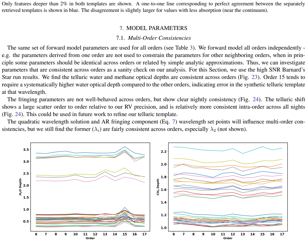
- The paper's finding that telluric optical depths are consistent across orders suggests that a future joint fit over all orders, sharing telluric and fringing parameters, could shrink the 48-parameter freedom and push precision below the current 3–5 m/s floor.
- Since the template is built from barycenter-shifted residuals, a testable requirement is that each target be observed at enough epochs spread over the year; one could derive a minimum-epoch criterion from the convergence behavior, something the paper does not quantify.
Signed reviews
Editorial analysis
A structured set of objections, weighed in public.
Referee Report
Summary. This manuscript describes a new data-analysis pipeline for extracting radial velocities from K-band (2.18-2.47 μm) spectra taken with iSHELL at the IRTF. The pipeline forward-models each echelle order with 48 parameters: a 13CH4 gas-cell transmission, four telluric absorbers, two fringing sources (OS filter and AR coating), a residual blaze, a Hermite-polynomial LSF, a wavelength solution with spline corrections, and an iteratively retrieved stellar template. RVs are combined across orders using weighted statistics or a TFA-like detrending minimization. Applying the pipeline to Barnard's Star, GJ 15 A, and 61 Cygni A, the authors report best-case long-term RV RMS values of 4.3, 2.7, and 3.8 m/s, respectively, after selecting a subset of orders by a powerset search and, for 61 Cyg A, discarding one night with a +1 km/s outlier. The paper claims 5 m/s precision over one-year baselines for two stars and 3 m/s over one month for GJ 15 A, and argues that this enables TESS planet confirmation around K and M dwarfs.
Significance. The manuscript's contribution, if the claimed precision is externally validated, is significant: it would make iSHELL one of the few instruments delivering few-m/s RVs in the K band using a Cassegrain-mounted spectrograph and a methane isotopologue gas cell, with public data. The forward-model architecture is detailed, and the inclusion of multiple fringing sources and iterative template retrieval is technically ambitious. The paper also makes honest statements about its limitations, including template corruption, uncharacterized telluric error, and order-selection freedom. The main weakness is that the headline numbers are internal, best-case metrics rather than predictive, externally anchored benchmarks: the stellar template is derived from the same spectra, the order subset is chosen post hoc, and no known planetary signal is recovered. Consequently, the paper currently demonstrates internal consistency and a plausible precision floor, but not that real RV signals at the few-m/s level survive the pipeline. If the recommended external-validation tests are added, this would be a valuable instrument-paper for TESS follow-up.
major comments (4)
- [Section 5.1, Table 5, Fig. 8] The headline precision values are minima of a powerset search over order combinations. For Barnard's Star (high SNR), the reported 4.33 m/s is the minimum of 4083 combinations; for GJ 15 A, 2.72 m/s comes from only three orders (8, 9, 10) and six nights; for 61 Cyg A, 3.77 m/s comes from five orders. A minimum over a large set is an optimistically biased statistic and is not a prediction of the precision obtained when the order set is fixed in advance. The authors partially acknowledge this at the end of Section 5.2 ('when observing stars with unknown RVs, we do not have this freedom'), but the Abstract and Section 5.1 still present the best-case values as the demonstrated precision. Additionally, the best single-order precisions in Table 4 are quoted at order-dependent 'best iteration' values, and it is unclear whether the multi-order subsets use different iterations per order, which adds further post-hoc freedom. I recommend reporting the full distribution of σ over the powerset or quoting a pre-specified fixed-order precision (e.g., the 5-7 m/s for at least 8 orders mentioned in Section 5.2) as the primary claim.
- [Section 4.3, Eq. (1), Table 5] The stellar template is constructed iteratively from the same target spectra, and the authors themselves state that 'residual correlated noise can gradually get repeatedly added into the stellar template from missed bad pixels, or from non-stellar spectral features that are not well fit.' This creates a circularity for the precision claim: low scatter of RVs relative to a template that may have absorbed some of the correlated signal does not prove that real, time-variable stellar velocities are preserved. The seasonal template comparison in Section 6 checks consistency of deep stellar lines, but it does not test whether signals at the few-m/s level survive. Because GJ 15 A is listed in Table 1 as hosting a planet with K=2.9 m/s and P=11.44 d, the paper should attempt to recover this known signal (e.g., by fitting the six nights to the published ephemeris or showing an RV periodogram) as an external validation. Barnard's Star's 233-day, 1.2 m/s signal is smaller but could also be checked. Without such a test, the m/s claim remains an internal precision metric rather than a demonstrated capability to detect or confirm planets.
- [Section 2 and Section 5.2] Telluric error is explicitly uncharacterized. The text states 'we do not characterize this' regarding water vapor variability and, in Section 5.2, 'Determining telluric induced error on RVs is the subject of a future investigation.' The K-band orders contain deep, variable water and methane lines; the forward model has four telluric species with a shared velocity shift; and order 14 is flagged as an outlier for all three targets, suggesting a telluric or gas-cell template problem. Since telluric absorption is a major potential contributor to the m/s error budget, the paper needs at least an upper-limit estimate, for example comparing RVs from orders with high versus low telluric absorption or injecting synthetic telluric variations. Until then, the claim that the achieved precision is below the telluric noise floor is unsupported.
- [Section 5.1, Table 5 (61 Cyg A)] The night JD 263.01044249 with RV = 1403 m/s is discarded on the assumption that it is an observational error or a flare, with no independent evidence. This exclusion is load-bearing for the '3.8 m/s for 61 Cyg A' claim. The paper should state the RMS with and without this night and ideally investigate the cause (e.g., checking target acquisition, flat fields, or telluric residuals). Also, the phrase 'over one year timescales' for 61 Cyg A is based on 10 nights spanning about 254 days after the exclusion; the effective baseline and number of epochs should be stated explicitly.
minor comments (6)
- [Table 3] Row 10 labels the 'OS Filter Fringing Finesse' as 'FAR' but the symbol for the OS fringing finesse should be 'FOS' to match Eq. (5); 'FAR' is already used for the AR fringing finesse in row 15.
- [Section 4.3] The first paragraph contains the duplicated phrase 'which can which can'; this should be corrected.
- [Section 5.2, Eq. (17)] The reduced chi-squared values of 0.5-0.8 in Table 5 are computed using uncertainties that themselves come from the forward model; a sentence clarifying that these values do not independently validate the error bars would prevent over-interpretation.
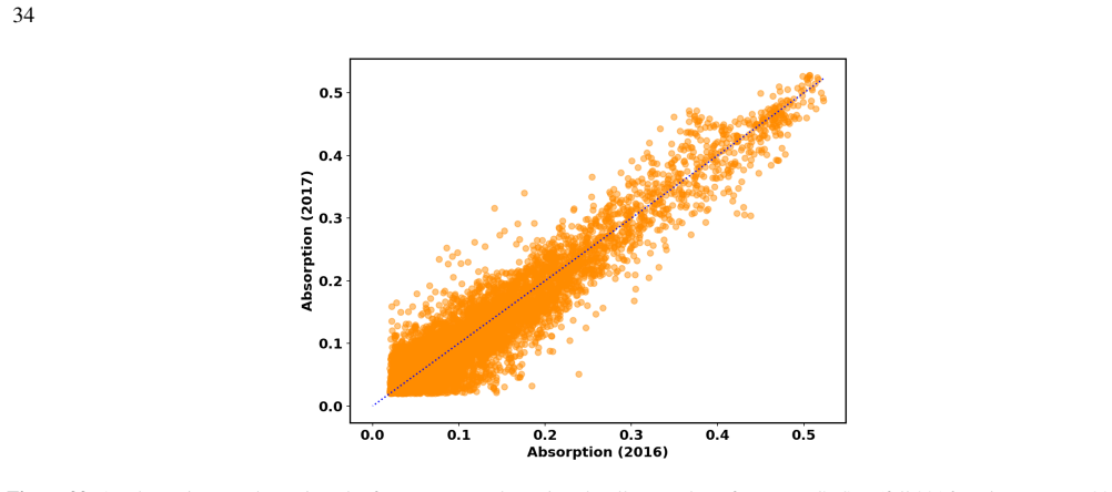
- [Section 6] The comparison of the two seasonal templates is qualitative only; reporting a quantitative metric (e.g., RMS difference over pixels with line depth >2%) would make the assessment more reproducible.
- [Figure 8] The caption should explicitly state that the yellow histogram includes combinations of 2-12 orders while the green histogram is restricted to 10-12 orders; the current caption relies on the main text for this information.
- [Reproducibility] The core pipeline PySHELL is listed as 'Available upon request' rather than deposited in a public repository; making it available publicly, as was done for the reduction code, would strengthen the reproducibility of the results.
Circularity Check
No circular derivation: the m/s claim is an in-sample self-calibration statistic, with overfitting and template-fidelity risks but no input-output identity.
full rationale
The paper's headline precision is the scatter of nightly RVs measured against a stellar template that is itself retrieved from the same observations (Sec. 4.3: 'we choose to rely on the target observations themselves to extract the stellar spectrum using an iterative deconvolution method'). This is a self-calibration, not a circular reduction: the forward model minimizes per-spectrum RMS residuals, not the long-term RV RMS, and the template does not by construction force the nightly scatter to zero. Per-order means are subtracted before combining (Eqs. 11-12), so only the constant zero-point is removed, which is standard for relative RVs. The powerset order selection in Sec. 5.1 ('looking at all possible values of sigma_RV from the powerset') is an in-sample best-case choice; the paper explicitly labels it 'best case' and separately quotes 5-7 m/s for configurations with at least 8 orders, so the best value is not being renamed as an out-of-sample prediction. The seasonal template comparison in Sec. 6 and the photon-noise estimates provide independent checks of internal consistency, even though they do not prove that real time-variable signals survive at the m/s level. The deferred derivation of the AR fringing model (Eq. 7, 'Cale et al. in prep') is an omitted proof, not a circular step. No load-bearing argument reduces to a self-citation, and no equation in the paper is identical to its input by construction. Residual concerns about template absorption of correlated noise and order-selection optimism are correctness and external-validation issues, not circularity.
Assumptions & free parameters
free parameters (9)
- Per-spectrum stellar Doppler shift v_star =
unbounded, output RVs
- Multi-order subset selection (powerset) =
e.g., orders 7-9, 11, 13 for Barnard's Star high-SNR run
- Telluric optical depths (H2O, CH4, N2O, CO2) =
bounds: 0.02-4.0, 0.1-3.0, 0.05-3.0, 0.05-3.0
- OS and AR fringing parameters (amplitudes, cavity scales, phase, finesse) =
bounds in Table 3
- LSF width a0 and 6 Hermite coefficients =
a0 bounds 5.5-12, aj +/-0.4
- Wavelength solution Lagrange points and 7 spline points =
3 quadratic points +/-0.05 nm, 7 splines +/-0.0125 nm
- Blaze function quadratic terms and 14 spline corrections =
b0 0.98-1.08, splines +/-0.135
- Stellar template (iteratively retrieved function) =
not a scalar; derived from target spectra
- TFA per-night and per-order offsets RV'_i and RV'_m =
bounds +/-50 and +/-5 m/s
assumptions (6)
- domain assumption Telluric templates from TAPAS with Maunakea T/P profile for April 12, 2018, 'arbitrarily chosen', are accurate for all epochs
- domain assumption The 13CH4 gas cell FTS spectrum and optical depth tau_g=0.97 accurately represent the cell in the spectrograph beam
- domain assumption Iterative stellar template retrieval converges to the true unconvolved stellar spectrum
- ad hoc to paper The 61 Cygni A +1 km/s night is an observational error or flare and can be discarded
- domain assumption The two fringing models (OS and AR) capture all significant quasi-sinusoidal fringing
- domain assumption Barycentric correction using exposure midpoint is adequate despite lack of exposure meter
Cite this review
Pith. "Pith review of Precise Radial Velocities of Cool Low Mass Stars With iSHELL." pith.science (2026). https://pith.science/paper/3EWCGETH
@misc{pith2026190807560,
  author       = {Pith},
  title        = {Pith review of: Precise Radial Velocities of Cool Low Mass Stars With iSHELL},
  year         = {2026},
  howpublished = {\url{https://pith.science/paper/3EWCGETH}},
  note         = {Machine review of arXiv:1908.07560}
}
read the original abstract
The coolest dwarf stars are intrinsically faint at visible wavelengths and exhibit rotationally modulated stellar activity from spots and plages. It is advantageous to observe these stars at near infrared (NIR) wavelengths (1-2.5 microns) where they emit the bulk of their bolometric luminosity and are most quiescent. In this work we describe our methodology and results in obtaining precise radial velocity (RV) measurements of low mass stars using K-band spectra taken with the R~80,000 iSHELL spectrograph and the NASA Infrared Telescope Facility (IRTF) using a methane isotopologue gas cell in the calibration unit. Our novel analysis pipeline extracts RVs by minimizing the RMS of the residuals between the observed spectrum and a forward model. The model accounts for the gas cell, tellurics, blaze function, multiple sources of quasi-sinusoidal fringing, and line spread function of the spectrograph (LSF). The stellar template is derived iteratively using the target observations themselves through averaging barycenter-shifted residuals. We have demonstrated 5 ms^-1 precision over one year timescales for the M4 dwarf Barnard's Star and K dwarf 61 Cygni A, and 3 ms^-1 over a month for the M2 dwarf GJ 15 A. This work demonstrates the potential for iSHELL to determine dynamical masses for candidate exoplanets discovered with the NASA TESS mission, and to search for exoplanets orbiting moderately active and/or young K and M dwarfs.
Figures


Figures from the paper (28 more)





Reference graph
Works this paper leans on
-
[1]
Aigrain, S., Parviainen, H., Roberts, S., Reece, S., & Evans, T. 2017, MNRAS, 471, 759
work page 2017
- [2]
-
[3]
2011, in Astronomical Society of the Pacific Conference Series, V ol
Allard, F., Homeier, D., & Freytag, B. 2011, in Astronomical Society of the Pacific Conference Series, V ol. 448, 16th Cambridge Workshop on Cool Stars, Stellar Systems, and the Sun, ed. C. Johns-Krull, M. K. Browning, & A. A. West, 91
work page 2011
-
[4]
2010, arXiv e-prints, arXiv:1012.3754 Anglada-Escud´e, G., Plavchan, P., Mills, S., et al
Andrae, R., Schulze-Hartung, T., & Melchior, P. 2010, arXiv e-prints, arXiv:1012.3754 Anglada-Escud´e, G., Plavchan, P., Mills, S., et al. 2012, PASP, 124, 586 Anglada-Escud´e, G., Butler, R. P., Reiners, A., et al. 2013, Astronomische Nachrichten, 334, 184 Anglada-Escud´e, G., Amado, P. J., Barnes, J., et al. 2016, Nature, 536, 437 Arfken G., Weber H., H...
arXiv 2010
-
[5]
Bailey, III, J. I., White, R. J., Blake, C. H., et al. 2012, ApJ, 749, 16
work page 2012
- [6]
-
[7]
Barclay, T., Pepper, J., & Quintana, E. V . 2018, ApJS, 239, 2
2018
-
[8]
Basri, G., Walkowicz, L. M., Batalha, N., et al. 2010, ApJL, 713, L155
work page 2010
Show all 47 references
-
[9]
L., Seifahrt, A., Hartman, H., et al
Bean, J. L., Seifahrt, A., Hartman, H., et al. 2010, ApJ, 713, 410
2010
- [10]
-
[11]
L., Lallement, R., Ferron, S., Boonne, C., & Bodichon, R
Bertaux, J. L., Lallement, R., Ferron, S., Boonne, C., & Bodichon, R. 2014, A&A, 564, A46
2014
-
[12]
H., Charbonneau, D., & White, R
Blake, C. H., Charbonneau, D., & White, R. J. 2010, ApJ, 723, 684
2010
-
[13]
2001, A&A, 374, 733
Bouchy, F., Pepe, F., & Queloz, D. 2001, A&A, 374, 733
2001
-
[14]
P., Marcy, G
Butler, R. P., Marcy, G. W., Williams, E., et al. 1996, PASP, 108, 500
1996
-
[15]
2012, in American Astronomical Society Meeting Abstracts, V ol
Choi, J., Marcy, G., & Howard, A. 2012, in American Astronomical Society Meeting Abstracts, V ol. 219, American Astronomical Society Meeting Abstracts #219, 245.04
2012
-
[16]
J., Mahmud, N
Crockett, C. J., Mahmud, N. I., Prato, L., et al. 2011, ApJ, 735, 78 —. 2012, ApJ, 761, 164
2011
-
[17]
A., Anglada-Escude, G., Arriagada, P., et al
Fischer, D. A., Anglada-Escude, G., Arriagada, P., et al. 2016, PASP, 128, 066001
2016
-
[18]
2016, PASP, 128, 104501
Gao, P., Plavchan, P., Gagn´e, J., et al. 2016, PASP, 128, 104501
2016
-
[19]
2016, PASP, 128, 084504
Gopalan, G., Plavchan, P., van Eyken, J., et al. 2016, PASP, 128, 084504
2016
-
[20]
W., Marcy, G
Howard, A. W., Marcy, G. W., Fischer, D. A., et al. 2014, ApJ, 794, 51
2014
-
[21]
Hunter, J. D. 2007, Computing in Science & Engineering, 9, 90
2007
-
[22]
S., Ramsey, L
Jenkins, J. S., Ramsey, L. W., Jones, H. R. A., et al. 2009, ApJ, 704, 975
2009
-
[23]
2001, SciPy: Open source scientific tools for Python Kaeufl, H.-U., Ballester, P., Biereichel, P., et al
Jones, E., Oliphant, T., Peterson, P., et al. 2001, SciPy: Open source scientific tools for Python Kaeufl, H.-U., Ballester, P., Biereichel, P., et al. 2004, in Proc. SPIE, V ol. 5492, Ground-based Instrumentation for Astronomy, ed. A. F. M. Moorwood & M. Iye, 1218–1227 Kov´acs,...
2001
-
[24]
I., Crockett, C
Mahmud, N. I., Crockett, C. J., Johns-Krull, C. M., et al. 2011, ApJ, 736, 123
2011
-
[25]
2015, ApJ, 798, 63 45 Mart´ın, E
Harder, J. 2015, ApJ, 798, 63 45 Mart´ın, E. L., Guenther, E., Del Burgo, C., et al. 2010, in Astronomical Society of the Pacific Conference Series, V ol. 430, Pathways Towards Habitable Planets, ed. V . Coud´e du Foresto, D. M. Gelino, & I. Ribas, 181
2015
-
[26]
1995, Nature, 378, 355
Mayor, M., & Queloz, D. 1995, Nature, 378, 355
1995
-
[27]
S., Becklin, E
McLean, I. S., Becklin, E. E., Figer, D. F., et al. 1995, in Proc. SPIE, V ol. 2475, Infrared Detectors and Instrumentation for Astronomy, ed. A. M. Fowler, 350–358
1995
-
[28]
Diddams, S. A. 2019a, arXiv e-prints, arXiv:1902.02817
1902 arXiv
-
[29]
J., Anderson, T., Bender, C
Metcalf, A. J., Anderson, T., Bender, C. F., et al. 2019b, arXiv e-prints, arXiv:1902.00500
1902 arXiv
-
[30]
R., Irwin, J., Charbonneau, D., Berta-Thompson, Z
Newton, E. R., Irwin, J., Charbonneau, D., Berta-Thompson, Z. K., & Dittmann, J. A. 2016, ApJ, 821, L19
2016
-
[31]
2015, arXiv e-prints, arXiv:1503.01770
Plavchan, P., Latham, D., Gaudi, S., et al. 2015, arXiv e-prints, arXiv:1503.01770
2015 arXiv
-
[32]
P., Anglada-Escude, G., White, R., et al
Plavchan, P. P., Anglada-Escude, G., White, R., et al. 2013, in Proc. SPIE, V ol. 8864, Techniques and Instrumentation for Detection of Exoplanets VI, 88641J
2013
-
[33]
2016, in Proc
Rayner, J., Tokunaga, A., Jaffe, D., et al. 2016, in Proc. SPIE, V ol. 9908, Ground-based and Airborne Instrumentation for Astronomy VI, 990884 RECONS. 2018, RECONS Research Consortium on Nearby Stars
2016
-
[34]
L., Huber, K
Reiners, A., Bean, J. L., Huber, K. F., et al. 2010, ApJ, 710, 432
2010
-
[35]
A., et al
Reiners, A., Zechmeister, M., Caballero, J. A., et al. 2018, A&A, 612, A49
2018
-
[36]
2018, Nature, 563, 365
Ribas, I., Tuomi, M., Reiners, A., et al. 2018, Nature, 563, 365
2018
-
[37]
2015, ApJL, 805, L22
Robertson, P., Roy, A., & Mahadevan, S. 2015, ApJL, 805, L22
2015
-
[38]
2018, PASP, 130, 074502
Sameshima, H., Matsunaga, N., Kobayashi, N., et al. 2018, PASP, 130, 074502
2018
-
[39]
2002, PASJ, 54, 873
Sato, B., Kambe, E., Takeda, Y ., Izumiura, H., & Ando, H. 2002, PASJ, 54, 873
2002
-
[40]
U., Z¨angl, G., et al
Seifahrt, A., K¨aufl, H. U., Z¨angl, G., et al. 2010, A&A, 524, A11
2010
-
[41]
2012, PyKE: Reduction and analysis of Kepler Simple Aperture Photometry data, Astrophysics Source Code Library, ascl:1208.004
Still, M., & Barclay, T. 2012, PyKE: Reduction and analysis of Kepler Simple Aperture Photometry data, Astrophysics Source Code Library, ascl:1208.004
2012
-
[42]
2018, A&A, 614, A122
Tal-Or, L., Zechmeister, M., Reiners, A., et al. 2018, A&A, 614, A122
2018
-
[43]
2012, ApJS, 203, 10
Tanner, A., White, R., Bailey, J., et al. 2012, ApJS, 203, 10
2012
-
[44]
2019, MNRAS van Belle, G
Blackman, R. 2019, MNRAS van Belle, G. T., & von Braun, K. 2009, ApJ, 694, 1085
2019
-
[45]
A., et al
Vanderburg, A., Plavchan, P., Johnson, J. A., et al. 2016, MNRAS, 459, 3565
2016
-
[46]
A., Hawley, S
West, A. A., Hawley, S. L., Walkowicz, L. M., et al. 2004, AJ, 128, 426
2004
-
[47]
T., & Eastman, J
Wright, J. T., & Eastman, J. D. 2014, PASP, 126, 838 46 Software: ishell reduction (https://github.com/jgagneastro/ishell reduction), PySHELL (Available upon request), Scipy (Jones et al. 2001), Matplotlib, (Hunter 2007), barycentric vel.pro (Wright & Eastman 2014)
2014
Reviewed August 14, 2026 · model on record in the stance chip above.
Discussion (0). Continue with ORCID to comment.