REVIEW 3 major objections 4 minor 77 references
A search for long-lived particles in compressed supersymmetry excludes top squarks to 1100 GeV and wino-like neutralinos to 550 GeV.
Reviewed by Pith at T0; open to challenge. T0 means a machine referee read the full paper against a public rubric. the ladder, T0–T4 →
T0 review · deepseek-v4-flash
2026-08-03 22:54 UTC pith:3FMQJEG5
load-bearing objection New compressed LLP exclusion from CMS using low-pT displaced tracks; solid analysis, but the alpha_p optimization wording must be clarified before the limits are fully credible. the 3 major comments →
Search for long-lived particles using displaced vertices with low-momentum tracks in proton-proton collisions at sqrt{s} = 13 TeV
The pith
A machine-rendered reading of the paper's core claim, the machinery that carries it, and where it could break.
Core claim
The paper's central claim is that long-lived particles with small mass splittings can be efficiently detected by reconstructing displaced vertices from tracks with transverse momentum as low as 0.5 GeV, even when the decay products are soft. In the top squark NLSP model, the search excludes top squark masses less than 400–1100 GeV, and for the bino-wino NLSP model it excludes wino-like neutralino masses less than 220–550 GeV, with the exact bound depending on the mass difference, the mass, and the lifetime of the long-lived particle. The observed limits are the strongest reported for these two coannihilation scenarios.
What carries the argument
The key mechanism is a purely data-driven background estimation based on transfer factors. Events are divided into four 'planes' by the number of good tracks in the displaced vertex (0, 1, 2, or ≥3), and within each plane into regions by missing transverse momentum (pTmiss > 700 GeV) and vertex displacement significance (S_vtx_xy > 20). Transfer factors—ratios of event counts between planes—are measured at low pTmiss (200–400 GeV) and applied to high-pTmiss control regions to predict backgrounds in the signal regions; the S_vtx_xy distribution is taken from low-pTmiss data as a proxy. The signal reconstruction relies on the inclusive vertex finder tuned to accept low-momentum tracks with lar
Load-bearing premise
The background prediction relies on the assumption that the ratio of event counts between planes with different numbers of good tracks, and the fraction of events with high vertex displacement significance, are the same at low missing transverse momentum (200–400 GeV) as at high missing transverse momentum (>700 GeV).
What would settle it
Measure, in a dedicated high-pTmiss control sample with zero good tracks, the fraction of events that would have S_vtx_xy > 20 and compare it with the low-pTmiss proxy used in the paper; a statistically significant upward trend with pTmiss would mean the tight-plane background predictions are biased low, and the quoted exclusions would shrink.
If this is right
- The compressed stop coannihilation parameter space with Δm = 12–25 GeV is closed for stop masses up to 400–1100 GeV, depending on the branching fraction.
- The bino-wino coannihilation scenario with wino-like neutralino masses below 220–550 GeV is excluded for lifetimes around 0.2–200 mm.
- The transfer-factor background method can be applied to future LLP searches that need multiple exclusive signal regions with limited simulation.
- The result provides a target for Run 3 and future collider searches: extending the same low-momentum displaced-vertex strategy to higher masses and smaller mass gaps.
Where Pith is reading between the lines
- The same technique could be applied to non-SUSY hidden-sector models that produce compressed spectra, such as dark photon or exotic Higgs decays, where final-state particles are soft.
- A testable extension: measure the S_vtx_xy and track-count ratios as a function of pTmiss in the 0-good-track control plane with the full Run 3 dataset; any rising trend would indicate the transfer-factor prediction underestimates high-pTmiss backgrounds.
- The 10–11% track/vertex reconstruction systematic, inherited from a K0S control sample, might be reducible with better detector simulation, which would sharpen the exclusions.
- The low-pTmiss transfer factors assume no correlation between pTmiss and vertex multiplicity; if pileup conditions differ in later data-taking, the extrapolation should be revalidated.
Editorial analysis
A structured set of objections, weighed in public.
Referee Report
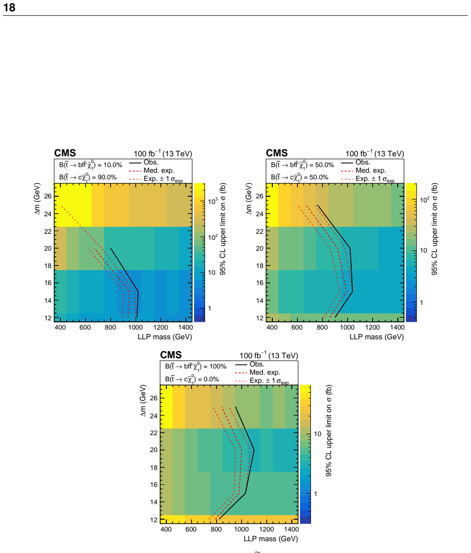
Summary. The paper reports a CMS search for long-lived particles (LLPs) in proton-proton collisions at 13 TeV using 100 fb^-1 of 2017-2018 data, targeting displaced vertices with low-momentum tracks, large missing transverse momentum, and an ISR jet. It interprets the search in two compressed-spectrum SUSY coannihilation benchmarks: a stop NLSP and a bino-wino NLSP with mass splittings of 12-25 GeV. The background is estimated entirely from data via a transfer-factor method that relates track-count planes and applies S_vtx_xy fractions measured at low pT_miss to the high-pT_miss signal regions. After a maximum-likelihood fit under the background-only hypothesis, the observed yields are consistent with the prediction (reported global p-value 0.5), and 95% CL limits are set excluding stop masses below 400-1100 GeV and bino-wino neutralino masses below 220-550 GeV depending on model parameters. The paper claims the most stringent limits to date for these two models and the first LHC sensitivity to such compressed LLP signatures using displaced vertices.
Significance. If the result holds, it closes a previously unexplored corner of LLP parameter space: compressed coannihilation scenarios with small mass splittings that have limited sensitivity in earlier displaced-vertex searches. The analysis is careful in several respects: the background estimate is data-driven with explicit transfer-factor equations; the SR-excluded material map is derived from data; the validation is performed in orthogonal planes; per-region discrepancies are reported transparently; and the tracking/vertexing efficiency is calibrated with K0S decays. These are substantive strengths. The main caveat is the optimization of the alpha_p selection: the text states it was optimized on 'event yields in the SRs' without clarifying whether those yields were observed or expected, and this ambiguity is load-bearing for the quoted exclusions. The transfer-factor closure also deserves quantitative support. With those points resolved, the result would meet the standard for a high-energy physics search paper.
major comments (3)
- [Section 4, alpha_p optimization] The text states: 'This threshold is optimized to maximize the search sensitivity based on the event yields in the SRs and is not directly derived from Fig. 4.' If 'event yields in the SRs' means the observed yields that are later fit under the background-only hypothesis and used for CLs limits, then the alpha_p > 0.2 requirement is a selection on the data being tested, which can bias the background-only p-value and inflate the quoted exclusion ranges in Figs. 10-11. The statement that the threshold is 'not directly derived from Fig. 4' does not resolve this. Please state explicitly whether the optimization used expected signal and background from simulation, blinded control regions, or observed SR yields; if the latter, the selection is circular and the limits should be rederived with a frozen/blinded threshold. The ambiguity must be removed before the central exclusion claim can be asse
- [Section 5, Eqs. (3)-(11) and Fig. 7] The transfer factors are measured in the 200 < pT_miss < 400 GeV range and applied at pT_miss > 700 GeV, relying on the asserted independence of pT_miss and S_vtx_xy and on track-count ratios being pT_miss-independent. The validation in Fig. 7 is described only qualitatively ('For most of the regions... agree within statistical uncertainties'), and the paper does not report a quantitative closure test or a validation p-value. The observed departures in the search planes (tight B/D: 3 and 5 observed vs. 7.7 and 9.2 predicted; medium B: 98 vs. 78.8) are acknowledged but not propagated into the limit coverage. Please provide a quantitative pT_miss-dependence check for the transfer factors, a validation p-value for the orthogonal planes, and an explicit statement of how the observed deviations affect the CLs expected/observed limits.
- [Section 6, K0S calibration] The K0S-based efficiency systematic is derived after normalizing simulation to data at small Lxy, so the 10-11% envelope covers the Lxy-shape dependence but by construction absorbs the absolute reconstruction efficiency. The paper does not separately quantify the absolute normalization uncertainty in the signal efficiency. Since the quoted cross-section limits scale directly with signal efficiency, please state what part of the absolute efficiency is constrained by simulation only and what additional uncertainty (if any) is assigned to that absolute normalization.
minor comments (4)
- [Eq. (1)] The decay width is given in units of cm^-1, while cτ is quoted in length units. Please clarify the natural-unit convention and the relation cτ = B/Γ, including factors of c if needed.
- [Section 5, independence statement] The statement that pT_miss and S_vtx_xy are 'statistically independent' and that S_vtx_xy shapes are consistent across pT_miss ranges is not backed by a figure or a numerical test. Please include the relevant distribution comparison or a quantitative test statistic.
- [Section 7, p-value] The global p-value of 0.5 is quoted without specifying which regions enter the test statistic or whether nuisance parameters are profiled. Please define the statistic and the region set used for this p-value.
- [Section 4, vertex alpha_p discrepancy] The text notes that data vertices tend to have larger alpha_p than simulation because of pileup mismodeling. Since alpha_p is explicitly used in the optimization, please comment on how this data/simulation discrepancy affects the choice of the alpha_p threshold and the robustness of the assumed background model.
Circularity Check
No significant circularity: the analysis uses data-driven background estimates from control regions with orthogonal validation, and the cited theory inputs are external.
full rationale
The paper's central claim is an experimental exclusion, and the derivation chain is not circular. The background in the signal regions is not taken from the same regions: transfer factors are measured in the low-pT sideband (200 < pT_miss < 400 GeV) and in control regions B0/D0/B1/D1 of the nominal planes, multiplied across good-track plane indices, and the S_vtx_xy fraction is taken from low-pT data. The method is cross-checked in orthogonal validation planes, with an observed p-value of 0.5. Signal efficiencies are not normalized to the SR data: the K0S study normalizes data/simulation at small Lxy only to extract a shape-ratio systematic uncertainty (10–11%), and the material map explicitly excludes events contributing to the SRs. The only sentence that could look like selection on observed data is the alpha_p>0.2 optimization statement; however, Section 3 states that 'Simulated background events are used solely for selection optimization and systematic uncertainty studies and are not employed in the search results', so the SR-yield-based optimization is not a data-fitted input. Theoretical cross sections used for exclusions come from external NNLO+NNLL calculations, and no load-bearing self-citation or ansatz-smuggling step is present.
Axiom & Free-Parameter Ledger
free parameters (4)
- alpha_p > 0.2 vertex selection threshold =
0.2
- SR-defining thresholds (pT_miss > 700 GeV, S_vtx_xy > 20) =
700 GeV / 20
- KS calibration normalization =
unstated (MC normalized to data at small Lxy)
- Material-map density threshold =
unstated
axioms (7)
- domain assumption pT_miss and S_vtx_xy are statistically independent for backgrounds; transfer factors and S_vtx_xy shapes measured at 200-400 GeV transfer to pT_miss > 700 GeV.
- domain assumption Vertex reconstruction efficiency measured with KS decays (alpha_p < 0.2, two-track) applies to signal vertices (alpha_p > 0.2, one or more good tracks including low-pT tracks).
- domain assumption The stop four-body decay-width parameterization of Ref. [1] (Eq. 1) correctly maps (m_stop, Delta m, B) to cTau.
- domain assumption NNLO+NNLL production cross sections (Ref. [53]) are correct to their quoted uncertainties.
- domain assumption GEANT4 simulation of the CMS detector, after KS-based correction, models displaced low-pT track and vertex reconstruction in signal events.
- domain assumption For the bino-wino model, only Z-mediated chi20 decays into fermion pairs are considered; H-mediated decays are ignored.
- standard math The CLs procedure with profile likelihood in COMBINE is the accepted statistical standard for setting exclusion limits.
read the original abstract
A search for long-lived particles using final states including a displaced vertex with low-momentum tracks, large missing transverse momentum, and a jet from initial-state radiation is presented. This search uses proton-proton collision data at a center-of-mass energy of 13 TeV collected by the CMS experiment at the CERN LHC in 2017 and 2018, with a total integrated luminosity of 100 fb$^{-1}$. This analysis adopts specific supersymmetric (SUSY) coannihilation scenarios as benchmark signal models, characterized by a next-to-lightest SUSY particle (NLSP) with a mass difference of less than 25 GeV relative to the lightest SUSY particle, assumed to be a bino-like neutralino. In the top squark ($\tilde{\mathrm{t}}$) NLSP model, the NLSP is a long-lived $\tilde{\mathrm{t}}$, while in the bino-wino NLSP scenario, the mass-degenerate NLSPs are a wino-like long-lived neutralino and a short-lived chargino. The search excludes top squarks with masses less than 400$-$1100 GeV and wino-like neutralinos with masses less than 220$-$550 GeV, depending on the signal parameters, including the mass difference, mass, and lifetime of the long-lived particle. It sets the most stringent limits to date for the $\tilde{\mathrm{t}}$ and bino-wino NLSP models.
Figures



Reference graph
Works this paper leans on
-
[1]
A. Delgado et al., “The light stop window”,Eur. Phys. J. C73(2013) 2370, doi:10.1140/epjc/s10052-013-2370-5,arXiv:1212.6847
Pith/arXiv arXiv 2013
-
[2]
Light stop decays: Implications for LHC searches
R. Gr ¨ober, M. M. M¨uhlleitner, E. Popenda, and A. Wlotzka, “Light stop decays: Implications for LHC searches”,Eur. Phys. J. C75(2015) 420, doi:10.1140/epjc/s10052-015-3626-z,arXiv:1408.4662
Pith/arXiv arXiv 2015
-
[3]
Probing bino-wino coannihilation at the LHC
N. Nagata, H. Otono, and S. Shirai, “Probing bino-wino coannihilation at the LHC”, JHEP10(2015) 086,doi:10.1007/JHEP10(2015)086,arXiv:1506.08206
Pith/arXiv arXiv 2015
-
[4]
G. F. Giudice and A. Romanino, “Split supersymmetry”,Nucl. Phys. B699(2004) 65, doi:10.1016/j.nuclphysb.2004.08.001,arXiv:hep-ph/0406088. [Erratum: doi:10.1016/j.nuclphysb.2004.11.048]
Pith/arXiv arXiv 2004
-
[5]
Signatures of long-lived gluinos in split supersymmetry
J. L. Hewett, B. Lillie, M. Masip, and T. G. Rizzo, “Signatures of long-lived gluinos in split supersymmetry”,JHEP09(2004) 070,doi:10.1088/1126-6708/2004/09/070, arXiv:hep-ph/0408248
Pith/arXiv arXiv 2004
-
[6]
Aspects of split supersymmetry
N. Arkani-Hamed, S. Dimopoulos, G. F. Giudice, and A. Romanino, “Aspects of split supersymmetry”,Nucl. Phys. B709(2005) 3, doi:10.1016/j.nuclphysb.2004.12.026,arXiv:hep-ph/0409232
Pith/arXiv arXiv 2005
-
[7]
Gluino decays in split supersymmetry
P . Gambino, G. F. Giudice, and P . Slavich, “Gluino decays in split supersymmetry”,Nucl. Phys. B726(2005) 35,doi:10.1016/j.nuclphysb.2005.08.011, arXiv:hep-ph/0506214
Pith/arXiv arXiv 2005
-
[8]
A. Arvanitaki, N. Craig, S. Dimopoulos, and G. Villadoro, “Mini-split”,JHEP02(2013) 126,doi:10.1007/JHEP02(2013)126,arXiv:1210.0555
Pith/arXiv arXiv 2013
-
[9]
Simply unnatural supersymmetry
N. Arkani-Hamed et al., “Simply unnatural supersymmetry”, 2012.arXiv:1212.6971
Pith/arXiv arXiv 2012
-
[10]
J. Fan, M. Reece, and J. T. Ruderman, “Stealth supersymmetry”,JHEP11(2011) 012, doi:10.1007/JHEP11(2011)012,arXiv:1105.5135
Pith/arXiv arXiv 2011
-
[11]
A stealth supersymmetry sampler
J. Fan, M. Reece, and J. T. Ruderman, “A stealth supersymmetry sampler”,JHEP07 (2012) 196,doi:10.1007/JHEP07(2012)196,arXiv:1201.4875
Pith/arXiv arXiv 2012
-
[12]
Theories with gauge mediated supersymmetry breaking
G. F. Giudice and R. Rattazzi, “Theories with gauge mediated supersymmetry breaking”, Phys. Rept.322(1999) 419,doi:10.1016/S0370-1573(99)00042-3, arXiv:hep-ph/9801271
Pith/arXiv arXiv 1999
-
[13]
P . Meade, N. Seiberg, and D. Shih, “General gauge mediation”,Prog. Theor. Phys. Suppl. 177(2009) 143,doi:10.1143/PTPS.177.143,arXiv:0801.3278. 22
Pith/arXiv arXiv 2009
-
[14]
Exploring general gauge mediation
M. Buican, P . Meade, N. Seiberg, and D. Shih, “Exploring general gauge mediation”, JHEP03(2009) 016,doi:10.1088/1126-6708/2009/03/016,arXiv:0812.3668
Pith/arXiv arXiv 2009
-
[15]
Echoes of a hidden valley at hadron colliders
M. J. Strassler and K. M. Zurek, “Echoes of a hidden valley at hadron colliders”,Phys. Lett. B651(2007) 374,doi:10.1016/j.physletb.2007.06.055, arXiv:hep-ph/0604261
Pith/arXiv arXiv 2007
-
[16]
Discovering the Higgs through highly-displaced vertices
M. J. Strassler and K. M. Zurek, “Discovering the Higgs through highly-displaced vertices”,Phys. Lett. B661(2008) 263,doi:10.1016/j.physletb.2008.02.008, arXiv:hep-ph/0605193
Pith/arXiv arXiv 2008
-
[17]
Phenomenology of hidden valleys at hadron colliders
T. Han, Z. Si, K. M. Zurek, and M. J. Strassler, “Phenomenology of hidden valleys at hadron colliders”,JHEP07(2008) 008,doi:10.1088/1126-6708/2008/07/008, arXiv:0712.2041
Pith/arXiv arXiv 2008
-
[18]
ATLAS Collaboration, “Search for long-lived, massive particles in events with displaced vertices and missing transverse momentum in √s= 13 TeV pp collisions with the ATLAS detector”,Phys. Rev. D97(2018) 052012,doi:10.1103/PhysRevD.97.052012, arXiv:1710.04901
Pith/arXiv arXiv 2018
-
[19]
ATLAS Collaboration, “Search for long-lived, massive particles in events with a displaced vertex and a muon with large impact parameter in pp collisions at √s=13 TeV with the ATLAS detector”,Phys. Rev. D102(2020) 032006, doi:10.1103/PhysRevD.102.032006,arXiv:2003.11956
Pith/arXiv arXiv 2020
-
[20]
CMS Collaboration, “Search for long-lived particles decaying to jets with displaced vertices in proton-proton collisions at √s=13 TeV”,Phys. Rev. D104(2021) 052011, doi:10.1103/PhysRevD.104.052011,arXiv:2104.13474
Pith/arXiv arXiv 2021
-
[21]
Search for long-lived particles using displaced jets in proton-proton collisions at √s=13 TeV
CMS Collaboration, “Search for long-lived particles using displaced jets in proton-proton collisions at √s=13 TeV”,Phys. Rev. D104(2021) 012015, doi:10.1103/PhysRevD.104.012015,arXiv:2012.01581
Pith/arXiv arXiv 2021
-
[22]
ATLAS Collaboration, “Search for long-lived, massive particles in events with displaced vertices and multiple jets in pp collisions at √s= 13 TeV with the ATLAS detector”, JHEP06(2023) 200,doi:10.1007/JHEP06(2023)200,arXiv:2301.13866
Pith/arXiv arXiv 2023
-
[23]
CMS Collaboration, “Search for long-lived particles using displaced vertices and missing transverse momentum in proton-proton collisions at √s=13 TeV”,Phys. Rev. D109 (2024) 112005,doi:10.1103/PhysRevD.109.112005,arXiv:2402.15804
Pith/arXiv arXiv 2024
-
[24]
CMS Collaboration, “Search for light long-lived particles decaying to displaced jets in proton-proton collisions at √s=13.6 TeV”,Rept. Prog. Phys.88(2025) 037801, doi:10.1088/1361-6633/adaa13,arXiv:2409.10806
Pith/arXiv arXiv 2025
-
[25]
Search for displaced leptons in proton-proton collisions at √s= 13 TeV
B. Cardwell, “Search for displaced leptons in proton-proton collisions at √s= 13 TeV”. PhD thesis, Ohio State U., 2021
2021
-
[26]
Statistical combination of ATLAS Run 2 searches for charginos and neutralinos at the LHC
ATLAS Collaboration, “Statistical combination of ATLAS Run 2 searches for charginos and neutralinos at the LHC”,Phys. Rev. Lett.133(2024) 031802, doi:10.1103/PhysRevLett.133.031802,arXiv:2402.08347
Pith/arXiv arXiv 2024
-
[27]
CMS Collaboration, “Combined search for electroweak production of winos, binos, higgsinos, and sleptons in proton-proton collisions at √s= 13 TeV”,Phys. Rev. D109 (2024) 112001,doi:10.1103/PhysRevD.109.112001,arXiv:2402.01888. References 23
Pith/arXiv arXiv 2024
-
[28]
HEPData record for this analysis
“HEPData record for this analysis”, 2024.doi:10.17182/hepdata.166009
-
[29]
The CMS experiment at the CERN LHC
CMS Collaboration, “The CMS experiment at the CERN LHC”,JINST3(2008) S08004, doi:10.1088/1748-0221/3/08/S08004
-
[30]
Development of the CMS detector for the CERN LHC Run 3
CMS Collaboration, “Development of the CMS detector for the CERN LHC Run 3”, JINST19(2024) P05064,doi:10.1088/1748-0221/19/05/P05064, arXiv:2309.05466
Pith/arXiv arXiv 2024
-
[31]
CMS Collaboration, “The CMS trigger system”,JINST12(2017) P01020, doi:10.1088/1748-0221/12/01/P01020,arXiv:1609.02366
Pith/arXiv arXiv 2017
-
[32]
Performance of the CMS Level-1 trigger in proton-proton collisions at √s=13 TeV
CMS Collaboration, “Performance of the CMS Level-1 trigger in proton-proton collisions at √s=13 TeV”,JINST15(2020) P10017, doi:10.1088/1748-0221/15/10/P10017,arXiv:2006.10165
Pith/arXiv arXiv 2020
-
[33]
Performance of the CMS high-level trigger during LHC Run 2
CMS Collaboration, “Performance of the CMS high-level trigger during LHC Run 2”, JINST19(2024) P11021,doi:10.1088/1748-0221/19/11/P11021, arXiv:2410.17038
Pith/arXiv arXiv 2024
-
[34]
Electron and photon reconstruction and identification with the CMS experiment at the CERN LHC
CMS Collaboration, “Electron and photon reconstruction and identification with the CMS experiment at the CERN LHC”,JINST16(2021) P05014, doi:10.1088/1748-0221/16/05/P05014,arXiv:2012.06888
Pith/arXiv arXiv 2021
-
[35]
CMS Collaboration, “Performance of the CMS muon detector and muon reconstruction with proton-proton collisions at √s=13 TeV”,JINST13(2018) P06015, doi:10.1088/1748-0221/13/06/P06015,arXiv:1804.04528
Pith/arXiv arXiv 2018
-
[36]
Description and performance of track and primary-vertex reconstruction with the CMS tracker
CMS Collaboration, “Description and performance of track and primary-vertex reconstruction with the CMS tracker”,JINST9(2014) P10009, doi:10.1088/1748-0221/9/10/P10009,arXiv:1405.6569
Pith/arXiv arXiv 2014
-
[37]
The CMS Phase-1 pixel detector upgrade
Tracker Group of the CMS Collaboration, “The CMS Phase-1 pixel detector upgrade”, JINST16(2021) P02027,doi:10.1088/1748-0221/16/02/P02027, arXiv:2012.14304
Pith/arXiv arXiv 2021
-
[38]
Track impact parameter resolution for the full pseudo rapidity coverage in the 2017 dataset with the CMS Phase-1 pixel detector
CMS Collaboration, “Track impact parameter resolution for the full pseudo rapidity coverage in the 2017 dataset with the CMS Phase-1 pixel detector”, CMS Detector Performance Summary CMS-DP-2020-049, 2020
2017
-
[39]
Particle-flow reconstruction and global event description with the CMS detector
CMS Collaboration, “Particle-flow reconstruction and global event description with the CMS detector”,JINST12(2017) P10003,doi:10.1088/1748-0221/12/10/P10003, arXiv:1706.04965
Pith/arXiv arXiv 2017
-
[40]
Technical proposal for the Phase-II upgrade of the Compact Muon Solenoid
CMS Collaboration, “Technical proposal for the Phase-II upgrade of the Compact Muon Solenoid”, CMS Technical Proposal CERN-LHCC-2015-010, CMS-TDR-15-02, 2015. doi:10.17181/CERN.VU8I.D59J
-
[41]
The anti-kT jet clustering algorithm
M. Cacciari, G. P . Salam, and G. Soyez, “The anti-kT jet clustering algorithm”,JHEP04 (2008) 063,doi:10.1088/1126-6708/2008/04/063,arXiv:0802.1189
Pith/arXiv arXiv 2008
-
[42]
M. Cacciari, G. P . Salam, and G. Soyez, “FastJet user manual”,Eur. Phys. J. C72(2012) 1896,doi:10.1140/epjc/s10052-012-1896-2,arXiv:1111.6097. 24
Pith/arXiv arXiv 2012
-
[43]
Pileup mitigation at CMS in 13 TeV data
CMS Collaboration, “Pileup mitigation at CMS in 13 TeV data”,JINST15(2020) P09018, doi:10.1088/1748-0221/15/09/P09018,arXiv:2003.00503
Pith/arXiv arXiv 2020
-
[44]
Jet energy scale and resolution in the CMS experiment in pp collisions at 8 TeV
CMS Collaboration, “Jet energy scale and resolution in the CMS experiment in pp collisions at 8 TeV”,JINST12(2017) P02014, doi:10.1088/1748-0221/12/02/P02014,arXiv:1607.03663
Pith/arXiv arXiv 2017
-
[45]
CMS jet algorithms performance in 13 TeV data
CMS Collaboration, “CMS jet algorithms performance in 13 TeV data”, CMS Physics Analysis Summary CMS-PAS-JME-16-003, 2016
2016
-
[46]
Identification of heavy-flavour jets with the CMS detector in pp collisions at 13 TeV
CMS Collaboration, “Identification of heavy-flavour jets with the CMS detector in pp collisions at 13 TeV”,JINST13(2018) P05011, doi:10.1088/1748-0221/13/05/P05011,arXiv:1712.07158
Pith/arXiv arXiv 2018
-
[47]
Jet flavour classification using DeepJet
E. Bols et al., “Jet flavour classification using DeepJet”,JINST15(2020) P12012, doi:10.1088/1748-0221/15/12/P12012,arXiv:2008.10519
Pith/arXiv arXiv 2020
-
[48]
Performance summary of AK4 jet b tagging with data from proton-proton collisions at 13 TeV with the CMS detector
CMS Collaboration, “Performance summary of AK4 jet b tagging with data from proton-proton collisions at 13 TeV with the CMS detector”, CMS Detector Performance Summary CMS-DP-2023-005, 2023
2023
-
[49]
CMS Collaboration, “Performance of missing transverse momentum reconstruction in proton-proton collisions at √s=13 TeV using the CMS detector”,JINST14(2019) P07004,doi:10.1088/1748-0221/14/07/P07004,arXiv:1903.06078
Pith/arXiv arXiv 2019
-
[50]
CMS Collaboration, “Performance of reconstruction and identification ofτleptons decaying to hadrons andν τ in pp collisions at √s=13 TeV”,JINST13(2018) P10005, doi:10.1088/1748-0221/13/10/P10005,arXiv:1809.02816
Pith/arXiv arXiv 2018
-
[51]
J. Alwall et al., “The automated computation of tree-level and next-to-leading order differential cross sections, and their matching to parton shower simulations”,JHEP07 (2014) 079,doi:10.1007/JHEP07(2014)079,arXiv:1405.0301
Pith/arXiv arXiv 2014
-
[52]
J. Alwall et al., “Comparative study of various algorithms for the merging of parton showers and matrix elements in hadronic collisions”,Eur. Phys. J. C53(2008) 473, doi:10.1140/epjc/s10052-007-0490-5,arXiv:0706.2569
Pith/arXiv arXiv 2008
-
[53]
W. Beenakker et al., “NNLL-fast: Predictions for coloured supersymmetric particle production at the LHC with threshold and Coulomb resummation”,JHEP12(2016) 133, doi:10.1007/JHEP12(2016)133,arXiv:1607.07741
Pith/arXiv arXiv 2016
-
[54]
Interactions of heavy stable hadronizing particles
A. C. Kraan, “Interactions of heavy stable hadronizing particles”,Eur. Phys. J. C37 (2004) 91,doi:10.1140/epjc/s2004-01997-7,arXiv:hep-ex/0404001
Pith/arXiv arXiv 2004
-
[55]
Interactions of coloured heavy stable particles in matter
R. Mackeprang and A. Rizzi, “Interactions of coloured heavy stable particles in matter”, Eur. Phys. J. C50(2007) 353,doi:10.1140/epjc/s10052-007-0252-4, arXiv:hep-ph/0612161
Pith/arXiv arXiv 2007
-
[56]
Merging meets matching in MC@NLO
R. Frederix and S. Frixione, “Merging meets matching in MC@NLO”,JHEP12(2012) 061,doi:10.1007/JHEP12(2012)061,arXiv:1209.6215
Pith/arXiv arXiv 2012
-
[57]
A new method for combining NLO QCD with shower Monte Carlo algorithms
P . Nason, “A new method for combining NLO QCD with shower Monte Carlo algorithms”,JHEP11(2004) 040,doi:10.1088/1126-6708/2004/11/040, arXiv:hep-ph/0409146. References 25
Pith/arXiv arXiv 2004
-
[58]
Matching NLO QCD computations with parton shower simulations: the POWHEG method
S. Frixione, P . Nason, and C. Oleari, “Matching NLO QCD computations with parton shower simulations: the POWHEG method”,JHEP11(2007) 070, doi:10.1088/1126-6708/2007/11/070,arXiv:0709.2092
Pith/arXiv arXiv 2007
-
[59]
NLO single-top production matched with shower in POWHEG:s- andt-channel contributions
S. Alioli, P . Nason, C. Oleari, and E. Re, “NLO single-top production matched with shower in POWHEG:s- andt-channel contributions”,JHEP09(2009) 111, doi:10.1088/1126-6708/2009/09/111,arXiv:0907.4076. [Erratum: doi:10.1007/JHEP02(2010)011]
Pith/arXiv arXiv 2009
-
[60]
A general framework for implementing NLO calculations in shower Monte Carlo programs: the POWHEG BOX
S. Alioli, P . Nason, C. Oleari, and E. Re, “A general framework for implementing NLO calculations in shower Monte Carlo programs: the POWHEG BOX”,JHEP06(2010) 043, doi:10.1007/JHEP06(2010)043,arXiv:1002.2581
Pith/arXiv arXiv 2010
-
[61]
Single-top Wt-channel production matched with parton showers using the POWHEG method
E. Re, “Single-top Wt-channel production matched with parton showers using the POWHEG method”,Eur. Phys. J. C71(2011) 1547, doi:10.1140/epjc/s10052-011-1547-z,arXiv:1009.2450
Pith/arXiv arXiv 2011
-
[62]
T. Sj ¨ostrand et al., “An introduction toPYTHIA8.2”,Comput. Phys. Commun.191(2015) 159,doi:10.1016/j.cpc.2015.01.024,arXiv:1410.3012
Pith/arXiv arXiv 2015
-
[63]
Parton distributions for the LHC Run II
NNPDF Collaboration, “Parton distributions for the LHC Run II”,JHEP04(2015) 040, doi:10.1007/JHEP04(2015)040,arXiv:1410.8849
Pith/arXiv arXiv 2015
-
[64]
Parton distributions from high-precision collider data
NNPDF Collaboration, “Parton distributions from high-precision collider data”,Eur. Phys. J. C77(2017) 663,doi:10.1140/epjc/s10052-017-5199-5, arXiv:1706.00428
Pith/arXiv arXiv 2017
-
[65]
Extraction and validation of a new set of CMS PYTHIA8 tunes from underlying-event measurements
CMS Collaboration, “Extraction and validation of a new set of CMS PYTHIA8 tunes from underlying-event measurements”,Eur. Phys. J. C80(2020) 4, doi:10.1140/epjc/s10052-019-7499-4,arXiv:1903.12179
Pith/arXiv arXiv 2020
-
[66]
GEANT4 Collaboration, “GEANT4—a simulation toolkit”,Nucl. Instrum. Meth. A506 (2003) 250,doi:10.1016/S0168-9002(03)01368-8
-
[67]
Sensitivity of robust vertex fitting algorithms
J. D’Hondt, P . Vanlaer, R. Fruhwirth, and W. Waltenberger, “Sensitivity of robust vertex fitting algorithms”,IEEE T rans. Nucl. Sci.51(2004) 2037, doi:10.1109/TNS.2004.832296
arXiv 2004
-
[68]
Displaced tracking and vertexing calibration using neutral K mesons
CMS Collaboration, “Displaced tracking and vertexing calibration using neutral K mesons”, CMS Detector Performance Summary CMS-DP-2024-010, 2024
2024
-
[69]
Measurement of the inelastic proton-proton cross section at √s=13 TeV
CMS Collaboration, “Measurement of the inelastic proton-proton cross section at √s=13 TeV”,JHEP07(2018) 161,doi:10.1007/JHEP07(2018)161,arXiv:1802.02613
Pith/arXiv arXiv 2018
-
[70]
CMS luminosity measurement for the 2017 data-taking period at√s= 13 TeV
CMS Collaboration, “CMS luminosity measurement for the 2017 data-taking period at√s= 13 TeV”, CMS Physics Analysis Summary CMS-PAS-LUM-17-004, 2018
2017
-
[71]
CMS luminosity measurement for the 2018 data-taking period at√s= 13 TeV
CMS Collaboration, “CMS luminosity measurement for the 2018 data-taking period at√s= 13 TeV”, CMS Physics Analysis Summary CMS-PAS-LUM-18-002, 2019
2018
-
[72]
PDF4LHC recommendations for LHC Run II
J. Butterworth et al., “PDF4LHC recommendations for LHC Run II”,J. Phys. G43(2016) 023001,doi:10.1088/0954-3899/43/2/023001,arXiv:1510.03865
Pith/arXiv arXiv 2016
-
[73]
The CMS statistical analysis and combination tool: COMBINE
CMS Collaboration, “The CMS statistical analysis and combination tool: COMBINE”, Comput. Softw. Big Sci.8(2024) 19,doi:10.1007/s41781-024-00121-4, arXiv:2404.06614. 26
Pith/arXiv arXiv 2024
-
[74]
Lectures on statistics in theory: Prelude to statistics in practice
R. D. Cousins, “Lectures on statistics in theory: Prelude to statistics in practice”, 2018. arXiv:1807.05996
Pith/arXiv arXiv 2018
-
[75]
Confidence level computation for combining searches with small statistics
T. Junk, “Confidence level computation for combining searches with small statistics”, Nucl. Instrum. Meth. A434(1999) 435,doi:10.1016/S0168-9002(99)00498-2, arXiv:hep-ex/9902006
Pith/arXiv arXiv 1999
-
[76]
Presentation of search results: The CL s technique
A. L. Read, “Presentation of search results: The CL s technique”,J. Phys. G28(2002) 2693, doi:10.1088/0954-3899/28/10/313
-
[77]
Squark and gluino production cross sections in pp collisions at√s= 13, 14, 33 and 100 TeV
C. Borschensky et al., “Squark and gluino production cross sections in pp collisions at√s= 13, 14, 33 and 100 TeV”,Eur. Phys. J. C74(2014) 3174, doi:10.1140/epjc/s10052-014-3174-y,arXiv:1407.5066. 27 A The CMS Collaboration Yerevan Physics Institute, Yerevan, Armenia A. Hayrapetyan, V . Makarenko , A. Tumasyan1 Institut f ¨ ur Hochenergiephysik, Vienna, A...
Pith/arXiv arXiv 2014
discussion (0)
Sign in with ORCID, Apple, or X to comment. Anyone can read and Pith papers without signing in.