LVM-GP: Uncertainty-Aware PDE Solver via coupling latent variable model and Gaussian process

Hao Wu; Ling Guo; Tao Zhou; Wenwen Zhou; Xiaodong Feng; Xiaoliang Wan

REVIEW 3 major objections 6 minor 51 references

LVM-GP: Uncertainty-Aware PDE Solver via coupling latent variable model and Gaussian process

T0 review · 3 major / 6 minor · reviewed 2026-08-06 · deepseek-v4-flash

Challenge this review Re-run · record.json Download PDF Read on arXiv ↗

Pith's one-line read The paper claims that blending a latent Gaussian process with a neural operator yields a PDE solver whose accuracy and uncertainty rival HMC-based Bayesian PINNs at far lower cost.

desk verdict A clearly specified new architecture for UQ in PDE solving whose central claim currently rests on single-run visuals and an unchecked heteroscedastic-noise assumption; worth a serious review with mandatory calibration and code. read the letter →

arxiv 2507.22493 v1 pith:3IXPD3DC submitted 2025-07-30 stat.ML cs.AIcs.LG

Xiaodong Feng , Ling Guo , Xiaoliang Wan , Hao Wu , Tao Zhou , Wenwen Zhou This is my paper

classification stat.MLcs.AIcs.LG

keywords Gaussianprocesslatentvariablemodelneuraloperatorphysics-informedmachinelearninguncertaintyquantificationforwardPDEprobleminversenoisydata

verification ladder T0 review T1 audit T2 compute T3 formal

The pith

A machine-rendered reading of the paper's core claim, the machinery that carries it, and where it could break.

The reading

This paper proposes LVM-GP, a probabilistic solver that treats the solution of a PDE as a stochastic field instead of a single function. The core move is to build a latent representation by blending a learnable deterministic feature with a Gaussian process prior, the blend controlled by a confidence function learned from data, and then to map that representation to the solution with a neural operator. The authors claim this combination captures functional dependencies efficiently and produces predictive means and uncertainty estimates competitive with Bayesian physics-informed neural networks sampled by HMC, while avoiding HMC's cost and avoiding the spurious oscillations they report for deep ensembles under limited noisy data. If the claim holds, it gives a practical way to attach reliable uncertainty to forward and inverse PDE solutions, including parameter and source inference, from scattered noisy sensors.

What carries the argument

The central object is the confidence-gated latent encoder $z(x)=\mathrm{diag}(m(x))\bar{z}(x)+\mathrm{diag}(1-m(x))z_0(x)$, where $z_0$ is a vector-valued Gaussian process prior and $m(x)$ is a learned confidence function in $[0,1]$. This single construction carries the argument: it converts 'how far is x from the training data' into a variance on the latent, and the GP prior supplies spatial correlation that a standard normal latent would lack. The decoder is a neural operator with integral layers (an FNO-type kernel, or alternatively a DeepONet-type branch–trunk structure), which maps the latent process to the mean solution; a learnable variance function completes the conditional Gaussian decoder. Physics enters through a loss that evaluates the differential operator on the mean latent output, with the noise field deliberately not differentiated, and a KL regularization term prevents the confidence function from collapsing the latent to a deterministic function.

What would settle it

Run a one-dimensional forward Poisson test with known spatially varying noise, e.g. $\sigma(x)=a+bx$, and compare the PDE residual computed from full stochastic samples $u=\mu_u+\sigma_u\omega$ against the residual computed from the mean $\mu_u$. If the mismatch is large enough to move the predicted mean out of the data's noise band, or if the reported coverage of the 2-standard-deviation intervals degrades sharply in regions of strong noise gradient, then the no-differentiation assumption fails and the central claim of calibrated uncertainty is falsified.

Watch

Extended reading notes

Core claim

LVM-GP models the PDE solution as a conditional Gaussian whose mean is the output of a neural operator applied to a latent function, and whose variance is a learnable (possibly input-dependent) noise field. The latent function itself is constructed as $z(x) = \mathrm{diag}(m(x))\,\bar{z}(x) + \mathrm{diag}(1-m(x))\,z_0(x)$, where $\bar{z}$ is a learned deterministic feature, $z_0\sim \mathcal{GP}(0,K)$ is a vector-valued Gaussian process with squared-exponential kernel, and $m(x)\in[0,1]$ is a confidence function that the model learns from data. Away from observed points $m(x)$ tends toward 0, so the latent (and hence the solution) becomes more uncertain; near data it tends toward 1 and the latent becomes deterministic. Physics is imposed softly: the PDE residual is computed by automatic differentiation of the mean field only, under the stated assumption that the additive noise term is not differentiated. Training maximizes a data log-likelihood minus a KL regularization term borrowed from the information-bottleneck idea, preventing the latent from collapsing to a deterministic map. The paper reports comparisons with HMC-based Bayesian PINNs and deep ensembles on 1D Poisson, porous-media, nonlinear Poisson, 2D diffusion-reaction, and contaminant source inversion problems.

Load-bearing premise

The load-bearing premise is that the additive noise field can be treated as spatially varying but is never differentiated in the PDE residual; if the true noise varies in space in a way that interacts with the differential operator, the physics constraint and the resulting uncertainty estimates are biased.

Editorial extensions

If this is right

For forward problems with noisy data, a single trained network returns both a solution field and a spatially varying uncertainty that grows in regions where the confidence function sees little data.
For inverse problems, unknown PDE parameters or source locations are inferred with uncertainty estimates, and the PDE constraint can propagate information into regions with no direct measurements, as the paper's extrapolation experiment demonstrates.
The method avoids Hamiltonian Monte Carlo sampling, so the claimed accuracy and uncertainty quantification come at a much lower computational cost than B-PINN-HMC.
Replacing the standard normal latent prior with a Gaussian process prior gives uncertainty that inherits spatial correlation, which the paper argues is more informative than standard latent-variable models.
Because the decoder can be either an FNO-type or DeepONet-type operator, the framework transfers across function-space architectures.

Reading between the lines

Editorial extensions of the paper, not claims the author makes directly.

Editorial inference: the confidence function $m(x)$ is effectively a learned data-sparsity map, so it could be reused as an acquisition function for active sensor placement, a use the paper does not discuss.
Editorial inference: the stated assumption that $\sigma_u(x)$ is not differentiated restricts the method to noise models whose spatial variation does not enter the PDE residual; for strongly heteroscedastic or oscillatory noise, one could test whether a version that includes the derivative term produces better-calibrated uncertainty.
Editorial inference: the revised regularization term (17) has a limit as $B\to\infty$ that the paper leaves open; connecting it to a Gaussian process posterior over the latent would give a principled way to set the trade-off parameter $\beta$ and the kernel hyperparameters.

Share X Bluesky LinkedIn Reddit HN

Editorial analysis

A structured set of objections, weighed in public.

Desk editor's note, referee report, and a circularity audit.

Desk Editor's Note

read the letter

Two things before anything else. The architecture is new: a confidence-aware interpolation between a deterministic neural feature and a GP prior, fed through a neural operator decoder, with physics in the loss. That specific combination isn't in the literature. And the paper is clearly written and honest about its own gaps—the conclusion explicitly says the well-posedness of the revised regularizer is open.

What it does well: the method is fully specified; the GP derivative computations in Appendix A are careful; the revised regularizer in Remark 3.3 that couples latent values across inputs is a real improvement over the standard per-input KL; the 6D source inversion is a nontrivial demonstration.

The big problem is the evidence for the central UQ claim. Everything rests on a handful of single runs, one or two tables, and visual plots. No calibration or coverage statistics, no repeated-seed variability, no code or data. For a paper whose headline is 'robust UQ', that's a thin basis. The authors should be asked to add quantitative calibration, repeated runs, and release code before this claim can be taken seriously.

Second, the sigma_u assumption after Eq. (10) is a real gap in presentation. The general formulation and Remark 3.2 allow heteroscedastic sigma_u(x), but the residual is computed only on z_L, which is exact only for constant sigma_u. All reported experiments use scalar sigma, so the numerical results are fine, but the method overclaims what it supports. The paper should either restrict to scalar sigma or give a worked heteroscedastic test and clarify what sigma_u represents. As written, it is ambiguous whether sigma_u is solution-process noise (then the residual is incomplete) or pure observation noise (then calling it aleatoric solution uncertainty is misleading).

The lack of theory is a minor issue because the authors admit it; I would not hold that against them for a first submission. The extrapolation example is nice but one case.

Send it to peer review. A careful referee can extract a solid contribution, but only if the authors do the calibration work and fix the sigma_u ambiguity. If a revision comes back without calibration or code, I'd lean reject. With those, it's a useful paper for anyone in SciML UQ.

Referee Report

3 major / 6 minor

Summary. The paper proposes LVM-GP, a physics-informed probabilistic framework for forward and inverse PDE problems with noisy data. The model encodes a latent field by interpolating between a deterministic feature network and a Gaussian process prior, with the interpolation controlled by a learned confidence function m(x); a neural-operator decoder maps the latent field to the solution mean, and Gaussian noise terms model aleatoric uncertainty. Physical constraints are imposed as soft losses on the residual of the latent mean. The method is demonstrated on 1D Poisson, porous-media flow, nonlinear Poisson, 2D diffusion-reaction, and a 6D source-inversion problem, with comparisons to B-PINN-HMC and deep ensembles.

Significance. If the central claims held, LVM-GP would offer a scalable alternative to B-PINN-HMC and deep ensembles for uncertainty quantification in PDE problems, with a novel confidence-aware encoder and a flexible neural-operator decoder. The paper contains several useful elements: a closed-form expression for the GP-aware regularizer in Remark 3.3, a Karhunen-Loève expansion for differentiating the GP prior, both FNO- and DeepONet-type decoder variants, and an extrapolation experiment. However, the manuscript provides no code, no calibration or repeated-seed statistics, and the heteroscedastic noise model is under-specified. The significance is therefore conditional: the architecture is interesting and plausible, but the empirical evidence for 'robust uncertainty quantification' is not yet convincing.

major comments (3)

[Section 3.2, Eq. (10)] The model defines u(x,ω_u) = z_L(x,ω_E) + σ_u(x;θ_u_σ)·ω_u_D and then states that σ_u is not differentiated with respect to x, so that N_x[u] = N_x[z_L]. This assumption is load-bearing: for the heteroscedastic σ_u(x) explicitly allowed in Remark 3.2, N_x[σ_u·ω_u_D] is generically nonzero (for a linear operator it equals (N_x σ_u)·ω_u_D), so the stochastic component of u does not satisfy the PDE and the f-likelihood in Eq. (12) is misspecified. All numerical experiments use scalar σ_u, so the heteroscedastic case advertised in Remark 3.2 is never tested. The paper should either restrict σ_u to be constant, include the missing derivative terms in the residual, or reclassify σ_u as observation noise that should not be propagated through the PDE; as written, the robust-UQ claim for heteroscedastic noise is unsupported.
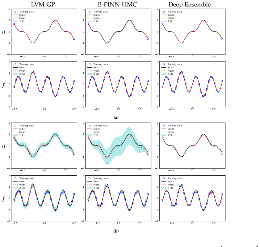
[Section 4, Tables 1–3 and Figures 4–10] The central claim of robust uncertainty quantification is supported only by single-run visual comparisons of mean ± 2 std bands and by mean/std tables for the inferred parameter λ. No calibration or coverage statistics (e.g., fraction of test points inside the reported credible intervals), no repeated-seed variability, and no quantitative uncertainty-quality metric are reported. For instance, in Table 1 at noise 0.01 the LVM-GP standard deviation for λ is 9.816×10^{-3}, more than twice the B-PINN-HMC value of 4.225×10^{-3}, and at noise 0.1 it is 6.954×10^{-2} versus 4.166×10^{-2}; without a calibration check the text's claim of 'tighter uncertainty estimation' in §4.1.1 cannot be distinguished from overconfidence. A proper evaluation requires repeated seeds, held-out test sets, and calibration diagnostics such as empirical coverage and interval scores.
[Section 3.2, Eqs. (13)–(15) and Remark 3.3] The KL regularizer actually optimized in the main objective uses e1(z) = N(0, I_dz), a standard normal, not the GP prior on z0. Since qE(z|x) is the marginal distribution at a single point x, this regularizer only shrinks each marginal toward an isotropic Gaussian and does not encode spatial correlations. The paper's stated contribution—that the GP prior 'captures spatial correlations across input locations, leading to more informed and structured uncertainty estimates' (Section 1)—is therefore not realized by the training objective used in most experiments. The revised regularizer in Eqs. (16)–(17) does use the GP covariance K, but it appears only in a Remark and is exercised only in the experiment of Figure 6. The authors should either use the GP-aware regularizer throughout, or temper the claim that the GP prior supplies structured uncertainty in the main method.

minor comments (6)

[Section 1, first paragraph] The phrase 'has remained an challenging scientific problem' should read 'has remained a challenging scientific problem'; the grammar as printed is broken.
[Section 3.2, Eq. (7)] The activation function and the noise standard deviations share the symbol σ (σ, σ_u, σ_f, σ_b). Using different symbols for the activation would remove avoidable confusion.
[Section 4.1.1, Figure 4] The horizontal axis of some u panels ranges from -0.5 to 0.5 while the f panels and the problem domain in Eq. (21) are on [-0.7, 0.7]; the panel limits should be made consistent.
[Section 4.1.1, Figure 5 and Section 4] The text states training runs for 10,000 iterations, but Figure 5's x-axis is labeled 'epoch' and reaches 20,000; reconcile the number of iterations and the axis label.
[Table 3] The rows labeled 'Std (×10^2)' and 'Std (×10^3)' are ambiguous; either report the actual standard deviations or clearly state which scaling factor applies to each entry.
[Algorithm 1 and Eq. (15)] Step 3 writes 'W = W + lr·∂L/∂W' while using the Adam optimizer, and Eq. (15) says to maximize L. Adam is conventionally a minimizer, so the algorithm should specify whether it minimizes -L or performs gradient ascent on L.

Circularity Check

0 steps flagged · score 0.0 of 10

No significant circularity: LVM-GP's uncertainty estimates come from a fitted probabilistic model with explicit priors and are benchmarked externally against B-PINN-HMC and deep ensembles.

full rationale

The paper's derivation chain is self-contained. The uncertainty estimates come from a learned encoder distribution q_E(z|x) = N(m(x) zbar(x), diag(1-m(x))^2), an explicit GP prior z0, and learned noise variances sigma_u, sigma_f (Eqs. (6)-(10) and (13)-(14)); these are parameters of a fitted model, not quantities claimed to be predicted from first principles. The only self-citation, [36] (IB-UQ), motivates the KL regularizer, but the paper derives L_reg explicitly from its own q_E(z|x) in Eqs. (13)-(14), so the citation is not load-bearing. The assumption after Eq. (10) that sigma_u(x) is not differentiated with respect to x is a modeling assumption that affects physical correctness for heteroscedastic noise (as acknowledged in Remark 3.2 and the conclusion's missing stability/well-posedness statement), but it is not circular: the residual and the f-likelihood are defined on mu_u by that explicit assumption. External comparisons against B-PINN-HMC and deep ensembles are reported on Poisson, porous-media, diffusion-reaction, and source-inversion problems, so the central accuracy and UQ claims are not reducible to the paper's own inputs.

Assumptions & free parameters 6 free parameters · 6 assumptions · 2 invented entities

The model introduces several learned or hand-set quantities; the most consequential are beta, the latent dimension, the GP length scale, and the noise scales, because they directly determine the width of the uncertainty bands. No new physical entities are proposed; the latent process and confidence function are internal modeling constructs without external falsifiable handles.

free parameters (6)

regularization weight beta = 0.01 (0.1 for extrapolation)
Chosen by hand; controls the trade-off between data fit and latent uncertainty, directly shaping the width of the uncertainty bands.
latent dimension d_z = 20
Fixed without a sensitivity study; determines the capacity of the latent Gaussian process.
GP kernel length scale L_c (or ell) = learned; 1D Poisson example stabilizes around 0.58
Learned during training (Section 4.1.1); controls the spatial correlation of the latent uncertainty process.
decoder noise std sigma_u, sigma_f, sigma_b = learnable scalars initialized at 2x empirical noise level
Fit to data; these aleatoric uncertainty estimates are not independently validated.
positional transformer kernel parameters alpha_i = parameterized as tan(alpha_tilde_i), learned
Learnable length scales in the decoder integral kernel (Eq. 8).
truncation level N in Karhunen-Loeve expansion = not specified explicitly
The GP prior is represented by a truncated KL expansion; truncation error affects both derivatives and the resulting uncertainty estimates.

assumptions (6)

domain assumption Observation noises are independent zero-mean Gaussians.
Eq. (5) assumes epsilon_u, epsilon_f, epsilon_b are independent zero-mean Gaussian noises; the likelihood is built on this assumption.
ad hoc to paper The aleatoric noise field sigma_u(x) is not differentiated with respect to x.
Stated just after Eq. (10); the PDE residual is computed only from the latent mean, excluding any spatial structure in the noise from the physics constraint.
ad hoc to paper The marginal prior e1(z) in the KL regularizer is standard normal.
Eq. (13) takes e1(z) ~ N(0, I_dz); the revised regularizer in Eq. (17) replaces this with a GP covariance, but the basic version is used in most experiments.
domain assumption The GP prior z0 has a squared exponential kernel with sigma_K = 1.
Section 3.2 fixes the kernel to a squared exponential with sigma_K = 1 and a length scale parameter; the representational adequacy of this kernel is not questioned.
standard math Mercer's theorem and term-by-term differentiation of the KL expansion are valid.
Appendix A uses Mercer's theorem and assumes sufficient smoothness of eigenfunctions to differentiate the GP pathwise; this is a standard but nontrivial functional-analytic assumption.
domain assumption The neural operator decoder is expressive enough to represent the PDE solution mapping.
The decoder is an FNO-type or DeepONet-type network; the paper relies on the universal approximation properties of such operators without proving rates for the specific stochastic mapping.

invented entities (2)

Confidence-aware latent process z1(x, omega)
purpose: Encodes input-dependent epistemic uncertainty by interpolating between a learned deterministic feature and a Gaussian process prior.
This is an internal modeling construct; there is no externally falsifiable handle, and its quality is only evaluated indirectly through predictive accuracy and uncertainty plots.
Confidence function m(x)
purpose: Controls the blend between the deterministic feature and the GP prior, with m near 1 at training data and m near 0 away from data.
Learned from data with no independent evidence outside the model; it directly sets the magnitude of latent uncertainty.

how reviews work

0 comments

Cite this review

Pith. "Pith review of LVM-GP: Uncertainty-Aware PDE Solver via coupling latent variable model and Gaussian process." pith.science (2026). https://pith.science/paper/3IXPD3DC

@misc{pith2026250722493,
  author       = {Pith},
  title        = {Pith review of: LVM-GP: Uncertainty-Aware PDE Solver via coupling latent variable model and Gaussian process},
  year         = {2026},
  howpublished = {\url{https://pith.science/paper/3IXPD3DC}},
  note         = {Machine review of arXiv:2507.22493}
}

read the original abstract

We propose a novel probabilistic framework, termed LVM-GP, for uncertainty quantification in solving forward and inverse partial differential equations (PDEs) with noisy data. The core idea is to construct a stochastic mapping from the input to a high-dimensional latent representation, enabling uncertainty-aware prediction of the solution. Specifically, the architecture consists of a confidence-aware encoder and a probabilistic decoder. The encoder implements a high-dimensional latent variable model based on a Gaussian process (LVM-GP), where the latent representation is constructed by interpolating between a learnable deterministic feature and a Gaussian process prior, with the interpolation strength adaptively controlled by a confidence function learned from data. The decoder defines a conditional Gaussian distribution over the solution field, where the mean is predicted by a neural operator applied to the latent representation, allowing the model to learn flexible function-to-function mapping. Moreover, physical laws are enforced as soft constraints in the loss function to ensure consistency with the underlying PDE structure. Compared to existing approaches such as Bayesian physics-informed neural networks (B-PINNs) and deep ensembles, the proposed framework can efficiently capture functional dependencies via merging a latent Gaussian process and neural operator, resulting in competitive predictive accuracy and robust uncertainty quantification. Numerical experiments demonstrate the effectiveness and reliability of the method.

Figures

Figures reproduced from arXiv: 2507.22493 by the authors.

**Figure 1.** The encoder structure of the proposed approach. In this work, we model the target solution u as a stochastic field. While conventional latent variable models introduce low-dimensional latent random variables to capture stochasticity, they often ignore potential spatial or functional correlations. Here, we model the latent variable as a high-dimensional stochastic process, providing a functional and infinite-dimensi… view at source ↗

**Figure 2.** LVM-GP for forward PDE problems. The input x is first processed by a confidence-aware encoder, which combines deterministic features ¯z and spatially varying uncertainty z0(x, ω) (defined by a Gaussian process) through a confidence function m. Then the latent representation z1(x; ω) is propagated through a deep integral operator, which models nonlinear mappings in function space and enables the representation of com… view at source ↗

**Figure 3.** LVM-GP for inverse PDE problem. The input x is first processed by a confidence-aware encoder, which combines deterministic features ¯z and spatially varying uncertainty z0(x, ω) (defined by a Gaussian process) through a confidence function m. Then the latent representation z1(x; ω) is propagated through a deep integral operator, which models nonlinear mappings in function space and enables the representation of comp… view at source ↗

Figures from the paper (7 more)

**Figure 4.** Figure 4: 1D Poisson equation. Predicted u and f from different methods with two data noise scales. (a) ϵf ∼ N(0, 0.012 ), ϵb ∼ N(0, 0.012 ). (b) ϵf ∼ N(0, 0.1 2 ), ϵb ∼ N(0, 0.1 2 ). 13 [PITH_FULL_IMAGE:figures/full_fig_p013_4.png]

**Figure 5.** Figure 5: 1D Poisson equation. Training dynamics of the hyperparameter in the Gaussian process prior. 0.7 0.0 0.7 2 1 0 1 2 Training data Exact Mean 2 Std 0.7 0.0 0.7 2 1 0 1 2 Training data Exact Mean 2 Std [PITH_FULL_IMAGE:figures/full_fig_p014_5.png]

**Figure 6.** Figure 6: 1D Poisson equation. Predicted u and f with learnable Lc, ϵu ∼ N(0, 0.1 2 ), ϵf ∼ N(0, 0.1 2 ). 4.1.2. 1D flow through porous media with boundary layer We now consider flows through a horizontal channel filled with a uniform porous medium governed by the following equa…

**Figure 7.** Figure 7: 1D flow through porous media with boundary layer. Predicted u from different methods with two data noise scales. (a) ϵg ∼ N(0, 0.012 ), ϵb ∼ N(0, 0.012 ). (b) ϵg ∼ N(0, 0.1 2 ), ϵb ∼ N(0, 0.1 2 ). 4.2. PDE inverse problem 4.2.1. 1D nonlinear Poisson equation We conside…

**Figure 8.** Figure 8: 1D nonlinear Poisson equation. Predicted u and f from different methods with two data noise scales. (a) ϵf ∼ N(0, 0.012 ), ϵb ∼ N(0, 0.012 ). (b) ϵf ∼ N(0, 0.1 2 ), ϵb ∼ N(0, 0.1 2 ). Noise scale LVM-GP B-PINN-HMC Deep Ensemble 0.01 Mean 0.6976 0.6967 0.6966 Std 9.816 …

**Figure 9.** Figure 9: Extrapolation of LVM-GP: predicted u and f with a limited number of observations on u. ϵu ∼ N(0, 0.012 ), ϵf ∼ N(0, 0.012 ). 4.2.2. 2D nonlinear diffusion-reaction system We consider the following PDE here k(∂ 2 x1 u + ∂ 2 x2 u) + λu 2 = f, x1, x2 ∈ [−1, 1], (23) where…

**Figure 10.** Figure 10: 2D nonlinear diffusion-reaction equation. Predicted errors and standard deviations for u from different methods with two data noise scales. (a) ϵf ∼ N(0, 0.012 ), ϵu ∼ N(0, 0.012 ). (b) ϵf ∼ N(0, 0.1 2 ), ϵu ∼ N(0, 0.1 2 ). 4.2.3. Six-dimensional source inverse proble…

Discussion (0). Sign in to comment.

Reference graph

Works this paper leans on

51 extracted references · 39 canonical work pages

[1]

G. E. Karniadakis, I. G. Kevrekidis, L. Lu, P . Perdikaris, S. Wang, L. Yang, Physics-informed machine learning, Nature Reviews Physics 3 (2021) 422–440

work page 2021
[2]

Willard, X

J. Willard, X. Jia, S. Xu, M. Steinbach, V . Kumar, Integrating scientific knowledge with machine learning for engineering and environmental systems, ACM Computing Surveys 55 (2022) 1–37

work page 2022
[3]

Machine Learning and Computational Mathematics

W. E, Machine learning and computational mathematics, arXiv preprint arXiv:2009.14596 (2020)

work page Pith review arXiv 2020
[4]

Raissi, P

M. Raissi, P . Perdikaris, G. E. Karniadakis, Physics-informed neural networks: A deep learning frame- work for solving forward and inverse problems involving nonlinear partial di fferential equations, Journal of Computational Physics 378 (2019) 686–707

2019
[5]

W. E, B. Yu, The deep Ritz method: A deep learning-based numerical algorithm for solving variational problems, Communications in Mathematics and Statistics 6 (2018)

work page 2018
[6]

Sirignano, K

J. Sirignano, K. Spiliopoulos, DGM: A deep learning algorithm for solving partial differential equations, Journal of computational physics 375 (2018) 1339–1364

work page 2018
[7]

Wang, J.-L

J.-X. Wang, J.-L. Wu, H. Xiao, Physics-informed machine learning approach for reconstructing reynolds stress modeling discrepancies based on DNS data, Physical Review Fluids 2 (2017) 034603

work page 2017
[8]

Raissi, A

M. Raissi, A. Yazdani, G. E. Karniadakis, Hidden fluid mechanics: Learning velocity and pressure fields from flow visualizations, Science 367 (2020) 1026–1030

work page 2020

Show all 51 references

[9]

J. Han, A. Jentzen, W. E, Solving high-dimensional partial di fferential equations using deep learning, Proceedings of the National Academy of Sciences 115 (2018) 8505–8510

2018
[10]

Huang, H

J. Huang, H. Wang, T. Zhou, An augmented Lagrangian deep learning method for variational problems with essential boundary conditions, Communications in Computational Physics 31 (2022) 966–986

2022
[11]

Y. Zang, G. Bao, X. Ye, H. Zhou, Weak adversarial networks for high-dimensional partial di fferential equations, Journal of Computational Physics 411 (2020) 109409

2020
[12]

L. Lu, P . Jin, G. Pang, Z. Zhang, G. E. Karniadakis, Learning nonlinear operators via Deeponet based on the universal approximation theorem of operators, Nature machine intelligence 3 (2021) 218–229. 21

2021
[13]

T. Chen, H. Chen, Universal approximation to nonlinear operators by neural networks with arbitrary activation functions and its application to dynamical systems, IEEE Transactions on Neural Networks 6 (1995) 911–917

1995
[14]

Z. Li, N. Kovachki, K. Azizzadenesheli, B. Liu, K. Bhattacharya, A. Stuart, A. Anandkumar, Fourier neural operator for parametric partial differential equations, arXiv preprint arXiv:2010.08895 (2020)

2020 arXiv
[15]

Cao, Choose a transformer: Fourier or galerkin, Advances in neural information processing systems 34 (2021) 24924–24940

S. Cao, Choose a transformer: Fourier or galerkin, Advances in neural information processing systems 34 (2021) 24924–24940

2021
[16]

Kissas, J

G. Kissas, J. H. Seidman, L. F. Guilhoto, V . M. Preciado, G. J. Pappas, P . Perdikaris, Learning operators with coupled attention, Journal of Machine Learning Research 23 (2022) 1–63

2022
[17]

S. Wang, H. Wang, P . Perdikaris, Learning the solution operator of parametric partial di fferential equations with physics-informed deeponets, Science advances 7 (2021) eabi8605

2021
[18]

S. Wang, H. Wang, P . Perdikaris, Improved architectures and training algorithms for deep operator networks, Journal of Scientific Computing 92 (2022) 35

2022
[19]

Geneva, N

N. Geneva, N. Zabaras, Modeling the dynamics of PDE systems with physics-constrained deep auto- regressive networks, Journal of Computational Physics 403 (2020) 109056

2020
[20]

A. F. Psaros, X. Meng, Z. Zou, L. Guo, G. E. Karniadakis, Uncertainty quantification in scientific machine learning: Methods, metrics, and comparisons, Journal of Computational Physics (2023) 111902

2023
[21]

Raissi, P

M. Raissi, P . Perdikaris, G. E. Karniadakis, Machine learning of linear di fferential equations using Gaussian processes, Journal of Computational Physics 348 (2017) 683–693

2017
[22]

Kendall, Y

A. Kendall, Y. Gal, What uncertainties do we need in bayesian deep learning for computer vision?, Advances in neural information processing systems 30 (2017)

2017
[23]

Y. Chen, B. Hosseini, H. Owhadi, A. M. Stuart, Solving and learning nonlinear PDEs with Gaussian processes, Journal of Computational Physics 447 (2021) 110668

2021
[24]

Y. Chen, H. Owhadi, F. Schäfer, Sparse cholesky factorization for solving nonlinear PDEs via Gaussian processes, arXiv preprint arXiv:2304.01294 (2023)

2023 arXiv
[25]

L. Yang, X. Meng, G. E. Karniadakis, B-PINNs: Bayesian physics-informed neural networks for forward and inverse PDE problems with noisy data, Journal of Computational Physics 425 (2021) 109913

2021
[26]

Linka, A

K. Linka, A. Schäfer, X. Meng, Z. Zou, G. E. Karniadakis, E. Kuhl, Bayesian physics informed neural networks for real-world nonlinear dynamical systems, Computer Methods in Applied Mechanics and Engineering 402 (2022) 115346

2022
[27]

G. Lin, C. Moya, Z. Zhang, B-DeepONet: An enhanced Bayesian DeepONet for solving noisy parametric pdes using accelerated replica exchange SGLD, Journal of Computational Physics 473 (2023) 111713

2023
[28]

Lotfi, P

S. Lotfi, P . Izmailov, G. Benton, M. Goldblum, A. G. Wilson, Bayesian model selection, the marginal likelihood, and generalization, in: International Conference on Machine Learning, PMLR, pp. 14223– 14247
[29]

Lakshminarayanan, A

B. Lakshminarayanan, A. Pritzel, C. Blundell, Simple and scalable predictive uncertainty estimation using deep ensembles, Advances in neural information processing systems 30 (2017)

2017
[30]

S. Fort, H. Hu, B. Lakshminarayanan, Deep ensembles: A loss landscape perspective, arXiv preprint arXiv:1912.02757 (2019)

2019 arXiv
[31]

Malinin, M

A. Malinin, M. Gales, Predictive uncertainty estimation via prior networks, Advances in neural information processing systems 31 (2018). 22

2018
[32]

Y. Yang, G. Kissas, P . Perdikaris, Scalable uncertainty quantification for deep operator networks using randomized priors, Computer Methods in Applied Mechanics and Engineering 399 (2022) 115399

2022
[33]

Amini, W

A. Amini, W. Schwarting, A. Soleimany, D. Rus, Deep evidential regression, Advances in Neural Information Processing Systems 33 (2020) 14927–14937

2020
[34]

Akhare, T

D. Akhare, T. Luo, J.-X. Wang, Diffhybrid-uq: uncertainty quantification for differentiable hybrid neural modeling, arXiv preprint arXiv:2401.00161 (2023)

2023 arXiv
[35]

P . Du, M. H. Parikh, X. Fan, X.-Y. Liu, J.-X. Wang, Conditional neural field latent di ffusion model for generating spatiotemporal turbulence, Nature Communications 15 (2024) 10416

2024
[36]

L. Guo, H. Wu, W. Zhou, T. Zhou, IB-UQ: Information bottleneck based uncertainty quantification for neural function regression and neural operator learning, arXiv preprint arXiv:2302.03271 (2023)

2023 arXiv
[37]

Bergna, S

R. Bergna, S. Depeweg, S. C. Ordonez, J. Plenk, A. Cartea, J. M. Hernandez-Lobato, Post-hoc uncertainty quantification in Pre-Trained Neural Networks via Activation-Level Gaussian Processes, arXiv preprint arXiv:2502.20966 (2025)

2025
[38]

A. S. Nair, B. Jacob, A. A. Howard, J. Drgona, P . Stinis, E-PINNs: Epistemic Physics-Informed Neural Networks, arXiv preprint arXiv:2503.19333 (2025)

2025
[39]

Z. Zou, X. Meng, A. F. Psaros, G. E. Karniadakis, NeuralUQ: A comprehensive library for uncertainty quantification in neural differential equations and operators, arXiv preprint arXiv:2208.11866 (2022)

2022 arXiv
[40]

Raissi, P

M. Raissi, P . Perdikaris, G. E. Karniadakis, Numerical gaussian processes for time-dependent and nonlinear partial differential equations, SIAM Journal on Scientific Computing 40 (2018) A172–A198

2018
[41]

D. Long, Z. Wang, A. Krishnapriyan, R. Kirby, S. Zhe, M. Mahoney, AutoIP: A united framework to integrate physics into Gaussian processes, in: International Conference on Machine Learning, PMLR, pp. 14210–14222
[42]

S. Fang, M. Cooley, D. Long, S. Li, R. Kirby, S. Zhe, Solving high frequency and multi-scale pdes with gaussian processes, arXiv preprint arXiv:2311.04465 (2023)

2023 arXiv
[43]

Zhong, H

W. Zhong, H. Meidani, PI-VAE: Physics-informed variational auto-encoder for stochastic di fferential equations, Computer Methods in Applied Mechanics and Engineering 403 (2023) 115664

2023
[44]

Garnelo, J

M. Garnelo, J. Schwarz, D. Rosenbaum, F. Viola, D. J. Rezende, S. Eslami, Y. W. Teh, Neural processes, arXiv preprint arXiv:1807.01622 (2018)

2018 arXiv
[45]

Cheng, O

N. Cheng, O. A. Malik, S. De, S. Becker, A. Doostan, Bi-fidelity variational auto-encoder for uncertainty quantification, Computer Methods in Applied Mechanics and Engineering 421 (2024) 116793

2024
[46]

L. Yang, D. Zhang, G. E. Karniadakis, Physics-informed generative adversarial networks for stochastic differential equations, SIAM Journal on Scientific Computing 42 (2020) A292–A317

2020
[47]

Y. Yang, P . Perdikaris, Adversarial uncertainty quantification in physics-informed neural networks, Journal of Computational Physics 394 (2019) 136–152

2019
[48]

J. Chen, K. Wu, Positional knowledge is all you need: Position-induced transformer (PiT) for operator learning, arXiv preprint arXiv:2405.09285 (2024)

2024 arXiv
[49]

Q. V . Le, A. J. Smola, S. Canu, Heteroscedastic Gaussian process regression, in: Proceedings of the 22nd international conference on Machine learning, pp. 489–496
[50]

Misra, Mish: A self regularized non-monotonic activation function, arXiv preprint arXiv:1908.08681 (2019)

D. Misra, Mish: A self regularized non-monotonic activation function, arXiv preprint arXiv:1908.08681 (2019)

2019 arXiv
[51]

Nobile, R

F. Nobile, R. Tempone, C. Webster, A sparse grid stochastic collocation method for partial di fferential equations with random input data, SIAM Journal on Numerical Analysis 46 (2008) 2309–2345. 23

2008

Pith tools

Reviewed August 6, 2026 · model on record in the stance chip above.

[1] [1]

G. E. Karniadakis, I. G. Kevrekidis, L. Lu, P . Perdikaris, S. Wang, L. Yang, Physics-informed machine learning, Nature Reviews Physics 3 (2021) 422–440

work page 2021

[2] [2]

Willard, X

J. Willard, X. Jia, S. Xu, M. Steinbach, V . Kumar, Integrating scientific knowledge with machine learning for engineering and environmental systems, ACM Computing Surveys 55 (2022) 1–37

work page 2022

[3] [3]

Machine Learning and Computational Mathematics

W. E, Machine learning and computational mathematics, arXiv preprint arXiv:2009.14596 (2020)

work page Pith review arXiv 2020

[4] [4]

Raissi, P

M. Raissi, P . Perdikaris, G. E. Karniadakis, Physics-informed neural networks: A deep learning frame- work for solving forward and inverse problems involving nonlinear partial di fferential equations, Journal of Computational Physics 378 (2019) 686–707

2019

[5] [5]

W. E, B. Yu, The deep Ritz method: A deep learning-based numerical algorithm for solving variational problems, Communications in Mathematics and Statistics 6 (2018)

work page 2018

[6] [6]

Sirignano, K

J. Sirignano, K. Spiliopoulos, DGM: A deep learning algorithm for solving partial differential equations, Journal of computational physics 375 (2018) 1339–1364

work page 2018

[7] [7]

Wang, J.-L

J.-X. Wang, J.-L. Wu, H. Xiao, Physics-informed machine learning approach for reconstructing reynolds stress modeling discrepancies based on DNS data, Physical Review Fluids 2 (2017) 034603

work page 2017

[8] [8]

Raissi, A

M. Raissi, A. Yazdani, G. E. Karniadakis, Hidden fluid mechanics: Learning velocity and pressure fields from flow visualizations, Science 367 (2020) 1026–1030

work page 2020