Who Wins Where? Conformal Model Comparison for Local Superiority

Baishi Li; Ke-Wei Huang; Xuan Yao; Yi Zhou

Local model superiority can be certified pointwise with finite-sample false-winner control: a winner is declared only when a one-sided conformal upper bound on a comparison score falls below zero.

Reviewed by Pith at T0; open to challenge. T0 means a machine referee read the full paper against a public rubric. the ladder, T0–T4 →

Challenge this review Re-run · record.json Download PDF Read on arXiv ↗

T0 review · deepseek-v4-flash

2026-08-03 14:33 UTC pith:3OUCBYEX

load-bearing objection A sound, honestly-scoped split-conformal procedure for local model comparison; the central guarantee is correct and the writing is clear, though the novelty is modest and the closest related work gets short shrift.

arxiv 2607.29053 v1 pith:3OUCBYEX submitted 2026-07-31 cs.LG

Who Wins Where? Conformal Model Comparison for Local Superiority

Yi Zhou , Baishi Li , Xuan Yao , Ke-Wei Huang This is my paper

classification cs.LG

keywords conformal predictionlocal model comparisonconditional mean scoresplit-sample inferencelocal winner mapbias-variance decompositionglobal-local mismatchmodel selection

verification ladder T0 review T1 audit T2 compute T3 formal T4 reserved

The pith

A machine-rendered reading of the paper's core claim, the machinery that carries it, and where it could break.

The paper argues that global model comparison—averaging losses across all covariates to pick one winner—can badly misrepresent where each model actually wins, and proposes a split-sample conformal procedure that maps local superiority instead. The central object is a conditional mean comparison score μ(x), such as the difference between two squared losses, and the main claim is that a local winner should be declared only when a one-sided conformal upper bound Ûα(x) is negative. This rule carries a finite-sample marginal guarantee: false winner declarations on the realized future score occur with probability at most α. The paper also shows that aggregate selection can disagree sharply with the prevalence of local winners, and that under squared loss the local score decomposes into squared-bias and variance differences, explaining mechanically where flexible versus structured models win.

Core claim

The paper establishes that a local best-model map can be made statistically honest: at any target covariate x, declare model A the local winner only when the locally centered conformal upper bound Ûα(x) is below zero. Under exchangeability of the calibration residuals and the future test residual conditional on the fitted models and local estimates, Proposition 1 guarantees that the probability of declaring a false winner—claiming A wins when the realized comparison score is nonnegative—is at most α in finite samples. The guarantee concerns the realized future score, not a confidence interval for μ(x), and it holds for any comparison score. The paper further proves asymptotic sign recovery

What carries the argument

The locally centered conformal upper bound is the central device. Three disjoint splits are used: one fits the competing models, one estimates a local center θ̂r(x) and scale σ̂r(x) from out-of-sample comparison scores, and one calibrates localized residuals to form the quantile q̂_{1−α}. The upper bound is θ̂r(x) + σ̂r(x)q̂_{1−α}, and the rule declares a winner only when this bound is negative. Exchangeability of calibration and test residuals conditional on the fitting and estimation splits is what delivers the finite-sample false-winner control, and the construction is deliberately agnostic to the choice of score function.

Load-bearing premise

The finite-sample guarantee holds only when the calibration residuals and the future test residual are exchangeable—that is, when the test point comes from the same distribution as the calibration data; under temporal drift or covariate shift, the stated false-winner control can fail.

What would settle it

Generate data with a temporal trend so that calibration points come from an early window and test points from a later window, then run the procedure and measure the empirical false-winner rate across many replications; if it systematically exceeds the nominal α, the exchangeability assumption is violated and the guarantee does not hold.

Watch this falsifier — get emailed when new claim-graph text bears on it.

If this is right

Practitioners can replace a single global winner with a spatially explicit best-model map whose false-winner declarations are bounded in finite samples.
The procedure abstains in regions of uncertainty and near tie boundaries, outputting a conservative certified subset rather than a forced winner map.
Because the conformal guarantee is score-agnostic, the same rule works for gap, log-ratio, or standardized scores, though efficiency and selection power vary.
Under squared loss, local winner regions are expected to coincide with regions where one model's squared-bias advantage overcomes its variance disadvantage.
Aggregate and local comparisons are logically independent: a model can be globally worse yet locally best for a large fraction of the population.

Where Pith is reading between the lines

These are editorial extensions of the paper, not claims the author makes directly.

Editorial: the same conformal machinery could extend to comparisons among multiple models or to local summary targets such as quantiles, though the paper's formal guarantee is stated for the realized future score of a pairwise comparison.
Editorial: the exchangeability requirement implies the method is safest in stationary settings; adapting it to covariate shift would require reweighted calibration, a natural testable extension.
Editorial: a practical consequence left implicit is that the certified winner map can serve as a routing rule at prediction time, but only if the marginal false-winner control is the accepted notion of risk.

Editorial analysis

A structured set of objections, weighed in public.

Desk editor's note, referee report, simulated authors' rebuttal, and a circularity audit.

Desk Editor's Note

A sound, honestly-scoped split-conformal procedure for local model comparison; the central guarantee is correct and the writing is clear, though the novelty is modest and the closest related work gets short shrift.

read the letter

Short version: this is a competent paper. The main result—split-conformal control of false local-winner declarations on the realized score—is a direct application of exchangeability, and the authors say so. They don't oversell it as a confidence statement about µ(x0). That restraint is the paper's best feature. The three-way split is clean, Proposition 1 is correct, and the proof is self-contained. Proposition 2 (global vs local prevalence) is elementary but worth stating, and Proposition 3 gives a clean bias-variance decomposition for squared loss.

What's actually new is the specific packaging: localized centering/scale before conformal calibration, plus the local winner-map framing. That's a legitimate extension, but it's not a conceptual leap. The paper would be stronger if it engaged with [11] directly—the related work mentions it but there's no empirical or theoretical comparison. Since [11] is about localized conformal model selection for interval efficiency, the objectives differ, but a reader wants to know when to use which.

Soft spots, in order: (1) the comparison to the closest paper is too thin; (2) the locality parameter k is heuristic and the ablation shows case-dependent behavior—that's fine but it means the method needs tuning; (3) Theorem 1 is stated for fixed-bandwidth kernels while experiments use KNN; the authors flag this, and the finite-sample guarantee doesn't depend on it, but the consistency theory doesn't exactly cover the deployed estimator; (4) the guarantee is marginal—again, acknowledged. None of these are load-bearing. The exchangeability limitation under drift is real but openly stated.

The experiments are small-scale but adequate: synthetic cases are designed to stress the mechanism, and the real-data results show the abstention behavior. Code is provided. The paper is not groundbreaking, but it is careful, readable, and correct. It deserves a serious referee and, with minor revisions, acceptance. I'd bring it to reading group and would cite it for the clean split-conformal comparison construction.

Referee Report

0 major / 6 minor

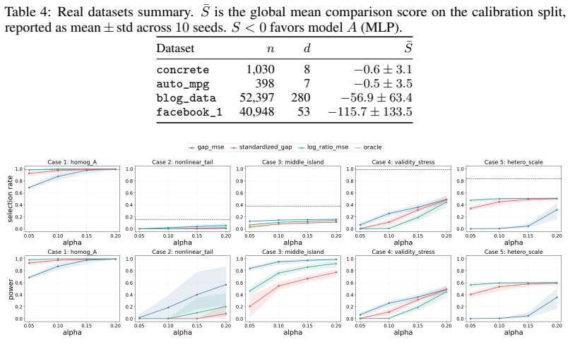
Summary. The paper introduces a split-sample conformal framework for local model comparison. Given two models and a comparison score S (e.g., squared-loss gap), it defines local targets: the conditional mean score μ(x), a finite-radius neighborhood average θ(x;r), and secondary majority/quantile summaries. The procedure uses three disjoint splits: a fitting split trains the models, an estimation split estimates the local center θ̂_r(x) and scale σ̂_r(x), and a calibration split computes localized residuals. For a test point, the conformal upper bound Û_α(x)=θ̂_r(x)+σ̂_r(x)q̂_{1−α} is formed, and model A is declared the local winner when Û_α(x)<0. Proposition 1 shows that under exchangeability of the calibration residuals and the test residual conditional on the fitting/estimation splits, P(S_{n+1}≤Û_α(X_{n+1}))≥1−α and P(Û_α(X_{n+1})<0, S_{n+1}≥0)≤α. Theorem 1 proves pointwise consistency of the local mean estimator away from tie boundaries under standard kernel conditions. Proposition 2 shows that aggregate selection can disagree sharply with local superiority prevalence. Proposition 3 gives a squared-loss bias–variance decomposition. Synthetic and real-data experiments validate the method's ability to recover heterogeneous winner regions, control false declarations, and achieve higher conditional gain than global selection.

Significance. The paper's central contribution is a principled, finite-sample valid method for local model comparison that complements global model selection. Proposition 1 is a correct application of split conformal prediction and is explicitly scoped to the realized future score, avoiding overclaiming. The paper is transparent that the guarantee is marginal and not a finite-sample confidence statement for μ(x). Theorem 1 and Proposition 3 are standard but useful for characterizing when local winners emerge. The paper ships reproducible code, and the empirical evaluation aligns with the theoretical guarantees, including the false-winner-rate control. The limitation section is candid about sample inefficiency, curse of dimensionality, marginality, and multiple comparisons. Overall, the central claim is sound and the paper is a solid contribution to the conformal prediction and model selection literature.

minor comments (6)

[Section 4 / Appendix A.1] The proof of Proposition 1 mentions 'using random tie-breaking only for the rank argument,' but the procedure does not specify random tie-breaking. The standard proof with q̂=R_{⌈(n+1)(1−α)⌉} can be stated directly with the usual empirical-quantile convention; please clarify to avoid ambiguity.
[Section 5.1 / Theorem 1] The consistency theorem is proved for fixed-bandwidth kernel localizers, while the experiments use KNN weights. The sentence 'The same applies to the estimation-split estimator in Section 4' would benefit from explicit conditions for KNN (e.g., k→∞, k/|Iest|→0) and a brief argument for the ratio estimator's consistency under those conditions. This gap does not affect Proposition 1, the main finite-sample result.
[Section 4 (p-value)] The one-sided conformal p-value p̂(x0) is presented without derivation. Please show the relationship between p̂(x0)≤α and the upper-bound rule Ûα(x0)<0, or at least clarify the rank convention. The claim that it is a 'slightly less conservative companion' then becomes easier to verify.
[Abstract / Section 1] The abstract says 'three disjoint splits,' but the experimental setup also uses a test split (four parts). Consider rewording to avoid confusion: the method itself uses three splits; a separate test set is used for evaluation.
[Section 6.1 / Figure 2] The caption says 'non-conformal methods can over-declare,' but it is not clear which non-conformal methods are shown in the plot. Specify the baselines so the comparison is reproducible.
[Section 3 / Section 6.1] The definitions local_def1, local_def2, and local_def3 are introduced in the experiments rather than in the formal setup. It would be clearer to define them in Section 3 alongside π_A and Q_{1−β} to connect the formal targets to the empirical rules.

Circularity Check

0 steps flagged

No significant circularity: the conformal guarantee and all theoretical results are derived from explicit exchangeability and definitional identities, not from fitted constants or self-citations.

full rationale

The paper's central result, Proposition 1, is a direct split-conformal rank argument. Conditional on the fitting and estimation splits, the localized center bθr and scale bσr are fixed measurable functions, and the calibration residuals together with the test residual are exchangeable. The proof in Appendix A.1 explicitly conditions on D0 and derives P(S_{n+1} ≤ Ûα) ≥ 1−α from the uniform rank of the test residual, then obtains the false-winner bound by the set inclusion {Ûα<0, S_{n+1}≥0} ⊆ {S_{n+1} > Ûα}. Nothing in this chain feeds the target back into the construction; the test point is held out and the fitted local quantities come from a disjoint estimation split. Proposition 2 is an existence construction showing that a distribution can have high local prevalence of A while the global mean favors B; this is a mathematical counterexample, not a prediction from fitted values. Proposition 3 is a bias–variance identity derived algebraically from the squared-loss decomposition and independence of training and test noise; the cancellation of the irreducible noise term follows from iterated expectation, not from the conclusion. Theorem 1 is a standard kernel-regression consistency proof. The paper also explicitly disclaims a finite-sample confidence statement for µ(x0), stating that Proposition 1 is 'intentionally phrased for the realized future score'. The limitations section acknowledges the exchangeability requirement and the marginal nature of the guarantee, which further delineates what is proven. No load-bearing self-citations appear; the cited conformal literature is external and standard. Overall, the derivation is self-contained and no circular step is present.

Axiom & Free-Parameter Ledger

3 free parameters · 4 axioms · 0 invented entities

The central claims rest on standard statistical assumptions: exchangeability for the conformal guarantee, i.i.d. sampling, and regularity conditions for the asymptotic consistency. The bias-variance decomposition assumes an additive noise model. No new theoretical entities are introduced.

free parameters (3)

locality parameter k = floor(sqrt(|Iest|)) in synthetic experiments; swept in ablation
Controls the neighborhood size for local estimation; not derived from theory, and optimal value is case-dependent.
regularization λ = not specified
Added to ensure the local scale is strictly positive; value not given in the text.
nominal level α = 0.10 in experiments
User-chosen significance level for the conformal bound.

axioms (4)

domain assumption Exchangeability of calibration and test residuals
Required for Proposition 1; stated in the proof, condition on D0.
domain assumption i.i.d. sample (X_i,Y_i)
Stated in Section 4 and used throughout.
domain assumption Regularity conditions for Theorem 1 (density, kernel, moments)
Standard nonparametric conditions, listed in Theorem 1.
domain assumption Additive noise model and independence of training/test for Proposition 3
Assumed at the start of Section 5.3.

pith-pipeline@v1.3.0-daily-deepseek · 14130 in / 13991 out tokens · 140059 ms · 2026-08-03T14:33:24.764732+00:00 · methodology

0 comments

read the original abstract

Standard model comparison is global, aggregating losses across the covariate space to declare a single winner. This can obscure heterogeneous performance, where different models are preferable in different regions. We introduce conformalized local model comparison, a split-sample framework for constructing calibrated local best-model maps. Given a model comparison score, such as the difference between two squared losses, the method uses three disjoint splits to fit competing models, estimate local centers and scales from out-of-sample scores, and conformally calibrate residual uncertainty. At a target point, the procedure declares a local winner only when a one-sided conformal bound excludes a tie, with the score's sign determining the favored model. We prove finite-sample marginal control for one-sided erroneous declarations on the realized future comparison score, establish pointwise consistency of the localized mean-score estimator away from tie boundaries, show that aggregate comparison can disagree sharply with the prevalence of local superiority, and derive a squared-loss bias--variance decomposition that clarifies how model structure affects local wins. Synthetic and real-data experiments show that the method recovers heterogeneous winner regions, abstains under uncertainty, and yields higher conditional gain than global selection.

Figures

Figures reproduced from arXiv: 2607.29053 by Baishi Li, Ke-Wei Huang, Xuan Yao, Yi Zhou.

**Figure 2.** Figure 2: False winner rate versus α. The diagonal marks the target level. Conformal methods control false winner declarations, while non-conformal methods can over-declare under noisy realized scores [PITH_FULL_IMAGE:figures/full_fig_p007_2.png] view at source ↗

**Figure 3.** Figure 3: Case 3 comparison between non-conformal local winner identification and conformal [PITH_FULL_IMAGE:figures/full_fig_p007_3.png] view at source ↗

**Figure 4.** Figure 4: Conformal selection versus α. Top: selection rate with the dashed line indicating the oracle A-winning rate. Bottom: oracle A power, P( ˆwα = A | µ(X) < −τ ), for the conformal methods [PITH_FULL_IMAGE:figures/full_fig_p008_4.png] view at source ↗

**Figure 5.** Figure 5: Bias–variance decomposition on Case 3. Left: [PITH_FULL_IMAGE:figures/full_fig_p008_5.png] view at source ↗

**Figure 7.** Figure 7: A/B winner regions in a 2D PCA projection. Colors show across-seed selection frequency: [PITH_FULL_IMAGE:figures/full_fig_p009_7.png] view at source ↗

**Figure 8.** Figure 8: Conditional gain versus selection rate on real datasets. Larger points correspond to a larger [PITH_FULL_IMAGE:figures/full_fig_p009_8.png] view at source ↗

**Figure 9.** Figure 9: Synthetic DGPs. Black dashed: f ⋆ (x); gray band: f ⋆ (x) ± 2σ(x); blue: a representative LightGBM (A) fit; red: linear (B) fit. B.4 Real datasets summary [PITH_FULL_IMAGE:figures/full_fig_p016_9.png] view at source ↗

**Figure 10.** Figure 10: Score-family ablation. Selection rate (top) and oracle [PITH_FULL_IMAGE:figures/full_fig_p018_10.png] view at source ↗

**Figure 11.** Figure 11: Locality parameter ablation. Selection rate (top) and oracle [PITH_FULL_IMAGE:figures/full_fig_p018_11.png] view at source ↗

**Figure 12.** Figure 12: Covariate-dimension ablation. horizontal axis is the ambient dimension [PITH_FULL_IMAGE:figures/full_fig_p018_12.png] view at source ↗

discussion (0)

Reference graph

Works this paper leans on

11 extracted references · 1 linked inside Pith

[1]

A. N. Angelopoulos and S. Bates. Conformal prediction: A gentle introduction.Foundations and Trends in Machine Learning, 16(4):494–591, 2023

2023
[2]

Giacomini and H

R. Giacomini and H. White. Tests of conditional predictive ability.Econometrica, 74(6):1545–1578, 2006

2006
[3]

L. Guan. Localized conformal prediction: A generalized inference framework for conformal prediction. Biometrika, 110(1):33–50, 2023

2023
[4]

M. I. Jordan and R. A. Jacobs. Hierarchical mixtures of experts and the EM algorithm.Neural Computation, 6(2):181–214, 1994

1994
[5]

J. Lei, M. G’Sell, A. Rinaldo, R. J. Tibshirani, and L. Wasserman. Distribution-free predictive inference for regression.Journal of the American Statistical Association, 113(523):1094–1111, 2018

2018
[6]

Liang, W

R. Liang, W. Zhu, and R. F. Barber. Conformal prediction after data-dependent model selection.arXiv preprint arXiv:2408.07066, 2024

Pith/arXiv arXiv 2024
[7]

Romano, E

Y . Romano, E. Patterson, and E. J. Candès. Conformalized quantile regression. InAdvances in Neural Information Processing Systems, 2019

2019
[8]

Shafer and V

G. Shafer and V . V ovk. A tutorial on conformal prediction.Journal of Machine Learning Research, 9: 371–421, 2008

2008
[9]

R. J. Tibshirani, R. F. Barber, E. J. Candès, and A. Ramdas. Conformal prediction under covariate shift. In Advances in Neural Information Processing Systems, 2019

2019
[10]

V ovk, A

V . V ovk, A. Gammerman, and G. Shafer.Algorithmic Learning in a Random World. Springer, 2005

2005
[11]

Wang and T

Y . Wang and T. Wang. Localized conformal model selection.arXiv preprint arXiv:2602.19284, 2026. 10 A Appendix: Proofs A.1 Proof of Proposition 1 Remark 1(Validity is agnostic to the score function).A fundamental property of split conformal prediction [10, 5] is that finite-sample marginal coverage relies on exchangeability of the calibration and test res...

arXiv 2026

[1] [1]

A. N. Angelopoulos and S. Bates. Conformal prediction: A gentle introduction.Foundations and Trends in Machine Learning, 16(4):494–591, 2023

2023

[2] [2]

Giacomini and H

R. Giacomini and H. White. Tests of conditional predictive ability.Econometrica, 74(6):1545–1578, 2006

2006

[3] [3]

L. Guan. Localized conformal prediction: A generalized inference framework for conformal prediction. Biometrika, 110(1):33–50, 2023

2023

[4] [4]

M. I. Jordan and R. A. Jacobs. Hierarchical mixtures of experts and the EM algorithm.Neural Computation, 6(2):181–214, 1994

1994

[5] [5]

J. Lei, M. G’Sell, A. Rinaldo, R. J. Tibshirani, and L. Wasserman. Distribution-free predictive inference for regression.Journal of the American Statistical Association, 113(523):1094–1111, 2018

2018

[6] [6]

Liang, W

R. Liang, W. Zhu, and R. F. Barber. Conformal prediction after data-dependent model selection.arXiv preprint arXiv:2408.07066, 2024

Pith/arXiv arXiv 2024

[7] [7]

Romano, E

Y . Romano, E. Patterson, and E. J. Candès. Conformalized quantile regression. InAdvances in Neural Information Processing Systems, 2019

2019

[8] [8]

Shafer and V

G. Shafer and V . V ovk. A tutorial on conformal prediction.Journal of Machine Learning Research, 9: 371–421, 2008

2008

[9] [9]

R. J. Tibshirani, R. F. Barber, E. J. Candès, and A. Ramdas. Conformal prediction under covariate shift. In Advances in Neural Information Processing Systems, 2019

2019

[10] [10]

V ovk, A

V . V ovk, A. Gammerman, and G. Shafer.Algorithmic Learning in a Random World. Springer, 2005

2005

[11] [11]

Wang and T

Y . Wang and T. Wang. Localized conformal model selection.arXiv preprint arXiv:2602.19284, 2026. 10 A Appendix: Proofs A.1 Proof of Proposition 1 Remark 1(Validity is agnostic to the score function).A fundamental property of split conformal prediction [10, 5] is that finite-sample marginal coverage relies on exchangeability of the calibration and test res...

arXiv 2026