REVIEW 5 major objections 8 minor 21 references
Patch-Based 3D Variational Autoencoder for Super-Resolution of Turbulent Channel Flow
T0 review · 5 major / 8 minor · reviewed 2026-08-06 · deepseek-v4-flash
Pith's one-line read A patch-based 3D variational autoencoder reconstructs fine turbulent structures from coarse flow fields, beating tricubic and Lanczos interpolation.
desk verdict The central methodology is self-contradictory, so the reported gains over interpolation cannot be trusted as described. read the letter →
The pith
A machine-rendered reading of the paper's core claim, the machinery that carries it, and where it could break.
The reading
What carries the argument
The load-bearing object is the patch-based 3D variational autoencoder: a 3D convolutional encoder maps a coarse $16^3$ input to a 16-dimensional Gaussian latent, and a 3D transposed-convolution decoder maps the latent back to a fine $16^3$ block. During inference the learned operator is applied convolutionally across the full domain with overlap averaging, so the parameter count scales with patch size rather than domain size. This patch strategy operationalizes the paper's locality hypothesis: the coarse neighborhood must carry enough information to determine the fine center.
What would settle it
Train the identical patch-based 3D-VAE on DNS data at a substantially different friction Reynolds number (say $Re_\tau \approx 2000$ or $5000$) and evaluate the held-out mean absolute error and FFT amplitude error; if they fall back to the tricubic or Lanczos levels, the local coarse-neighborhood assumption is the reason the original experiment succeeded.
Extended reading notes
Core claim
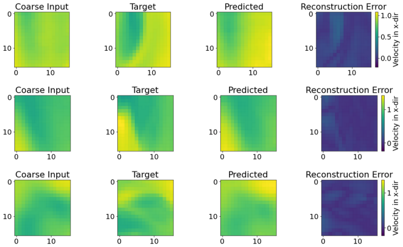
The central claim is that a patch-based 3D-VAE, trained on a single high-fidelity snapshot, learns an operator that reconstructs the central $16^3$ high-resolution block from a coarser neighborhood, and that this operator is a better super-resolver for turbulent channel flow than classical interpolation. The paper reports mean absolute errors below 0.06 for the streamwise velocity and a roughly threefold reduction in mean FFT amplitude error, and interprets this as evidence that the model restores small-scale spectral content rather than merely smoothing. The paper also extends the same model to coarse LES data and reports recovery of high-frequency modes absent in the input. It explicitly reports three limitations: attenuation of the smallest resolved scales, periodic artifacts caused by the patch stride, and under-prediction of extreme velocity values. The conditional 3D-GAN counterpart is described as a failed experiment under Wasserstein training.
Load-bearing premise
The load-bearing assumption is that a coarse-resolution view of a sufficiently large local region determines the fine-resolution flow at that region's center; if that local determinism fails, the patch-based model cannot be expected to generalize beyond its training flow.
Editorial extensions
If this is right
- If the central claim holds, learned super-resolution can recover turbulent spectral content that tricubic and Lanczos interpolation cannot, at roughly three times lower FFT amplitude error.
- Because the operator is applied patch-wise with overlapping average, full-domain super-resolution remains feasible even when the flow volume is much larger than the patch on which the model was trained.
- The reported transfer from filtered DNS to coarse LES inputs, if it generalizes, offers a way to enrich under-resolved simulations with fine-scale structure without running a second DNS.
- The paper's own limitations imply practical uses must account for smoothed smallest scales, periodic seam artifacts, and compressed extreme-velocity statistics.
- The failed Wasserstein-trained 3D-GAN leaves open which adversarial or hybrid losses, if any, can also stabilize 3D turbulence super-resolution.
Reading between the lines
- The locality assumption is untested across flow regimes: if small scales are instead governed by non-local pressure or transport effects that the patch context cannot see, the same architecture will likely degrade at other Reynolds numbers or geometries.
- The parameter-count-independence result suggests a natural extension to time-resolved super-resolution, where the same convolutional application could be run frame by frame, with temporal consistency as the open problem.
- A testable hybrid extension is to keep the VAE reconstruction but add a spectral or physics-based loss term targeting the attenuated smallest scales and extreme events named as limitations.
- The negative GAN result is itself informative: on this data the VAE's reconstruction loss plus probabilistic latent was sufficient, which suggests adversarial training may need stronger conditioning or domain-specific losses to add value.
Editorial analysis
A structured set of objections, weighed in public.
Referee Report
Summary. The paper proposes a patch-based 3D variational autoencoder (3D-VAE) for super-resolution of turbulent channel flow. The model is trained on a single DNS snapshot (timestamp 3200) from the Johns Hopkins Turbulence Database and evaluated on one held-out snapshot (timestamp 3280). The authors report that the VAE outperforms tricubic and Lanczos interpolation in mean absolute error (0.055 vs 0.075/0.076) and in a 2D FFT amplitude error (0.91 vs 2.63/2.85). A conditional 3D-GAN failed to converge and is reported as a negative result. The paper also describes an application to coarse LES-to-DNS super-resolution. The central hypothesis is that a coarse-resolution representation over a larger spatial context carries sufficient information to reconstruct a fine-resolution solution at the center of that region.
Significance. If the reported results are reproducible and the comparison is fair, the work would demonstrate that a learned patch-based operator can recover fine-scale turbulent structures beyond what standard interpolation achieves, with a parameter count independent of domain size. The paper also honestly reports a negative GAN result and acknowledges limitations such as attenuation of small scales and periodic artifacts. However, the current manuscript contains load-bearing contradictions in the patch-generation description and patch-assembly description, and the evaluation is extremely thin: errors are computed on a single X-Y plane of a single test snapshot with no error bars. These issues prevent the reader from assessing whether the central claim is actually supported. The paper also includes long sections on RANS/LES/VMS that are peripheral to the contribution.
major comments (5)
- [Section III-C]
- [Section IV vs Section VIII]
- [Section VI, Tables IX-X]
- [Section VI, baseline comparison]
- [Section VII]
minor comments (8)
- [Table I]
- [Section III-A]
- [Table V]
- [Section VI]
- [Section V]
- [Section III-D]
- [Sections I.A-I.C]
- [Figures]
Circularity Check
Patch-size formula makes the claimed 'larger context' self-definitional: q=A·s with the worked example q=16,A=4,s=4 makes the central 16^3 target equal the entire input cube, so the context advantage either vanishes or (under the 16^3-LR reading) is unspecified and uncompared.
-
self definitional
[Section III-C (Dataset Preparation, q = A·s and worked example); Section VIII (Conclusion hypothesis)]
"The cube size q is then defined as: q = A · s ... Example: Let A = 4 and s = 4, then: q = 4 · 4 = 16 ... The HR output is the central (16, 16, 16) portion of the original cube."
With q=16, the 'central (16,16,16)' target is the entire q-cube, so the supposedly 'larger coarse neighbourhood' is identical in spatial extent to the reconstructed block; the LR input is produced from the same 16^3 region (downsampled by stride A=4 to 4^3 and upsampled back to 16^3). Thus the stated hypothesis—that a coarse representation over a larger context reconstructs the center—is not implemented: there is no context outside the target. If one instead requires the LR cube to be 16^3, the formula forces s=16 and q=16A, but the paper never gives the actual q/s/A and the tricubic/Lanczos baselines are not given that outer context, so the comparison is uncontrolled. The advertised context advantage is an artifact of the patch-size definition, not a tested property.
full rationale
The core VAE experiment is otherwise a straightforward supervised fit: high-resolution DNS cubes are downsampled to form low-resolution inputs, the VAE is trained with reconstruction plus KL losses, and the numerical evaluation is performed on a temporally separated snapshot (timestamp 3280) rather than the training snapshot (3200). The MAE and FFT amplitude comparisons with tricubic and Lanczos interpolation are therefore not fits to the test set, and there are no load-bearing self-citations or imported uniqueness theorems. The principal circularity concern is the patch-geometry definition in Section III-C: the worked example makes the 'larger coarse neighbourhood' equal to the target region itself, so the central hypothesis in the Conclusion is not actually exercised. If the alternative reading is used (LR cube exactly 16^3, forcing s=16), the paper leaves q, s, and A unspecified and fails to give the interpolation baselines the same outer context, making the comparison uninterpretable. Additional internal contradictions—overlap averaging claimed in Section IV versus direct concatenation stated in the Conclusion—are consistency defects rather than circular reductions. Overall, one central design claim reduces to a definitional identity, but the learned mapping itself still has independent empirical content, giving a partial circularity score of 4.
Assumptions & free parameters
free parameters (4)
- latent dimension =
16
- coarsening factor A =
4
- patch stride s =
4
- training hyperparameters =
not reported
assumptions (3)
- domain assumption A coarse-resolution representation over a larger spatial context carries sufficient information to reconstruct a fine-resolution solution at the center.
- standard math The reparameterization trick in VAEs produces a differentiable estimator of the ELBO.
- ad hoc to paper A single DNS snapshot at Re_tau ~ 1000 is representative of turbulent channel flow statistics.
Cite this review
Pith. "Pith review of Patch-Based 3D Variational Autoencoder for Super-Resolution of Turbulent Channel Flow." pith.science (2026). https://pith.science/paper/3P72CIS7
@misc{pith2026250722082,
  author       = {Pith},
  title        = {Pith review of: Patch-Based 3D Variational Autoencoder for Super-Resolution of Turbulent Channel Flow},
  year         = {2026},
  howpublished = {\url{https://pith.science/paper/3P72CIS7}},
  note         = {Machine review of arXiv:2507.22082}
}
read the original abstract
Direct numerical simulation (DNS) accurately resolves all spatio-temporal scales of wall-bounded turbulence but becomes prohibitively expensive as the Reynolds number increases. Super-resolution (SR) provides a practical alternative by reconstructing fine-scale flow structures from coarse fields. Most existing SR methods focus on two-dimensional data, where vortex stretching is absent, and extend poorly to three dimensions because model complexity increases with the reconstructed volume. We propose a patch-based three-dimensional variational autoencoder (3D-VAE) that reconstructs a local (16^3) high-resolution block from a larger coarse neighbourhood. The learned operator is then applied convolutionally across the domain with overlap averaging, making the parameter count dependent only on patch size rather than domain size. The model is trained using the streamwise velocity from a single DNS snapshot of turbulent channel flow at (Re_\tau \approx 1000) from the Johns Hopkins Turbulence Database and evaluated on a held-out snapshot. Compared with DNS, the proposed method achieves a mean absolute error of 0.055, outperforming tricubic (0.075) and Lanczos (0.076) interpolation. In spectral space, it reduces the mean absolute error of the two-dimensional Fourier amplitude from 2.63 and 2.85 to 0.91, an improvement of about threefold. Applied to coarse finite-element simulations, the model reconstructs spectral content absent from the input, demonstrating transfer beyond filtered DNS. A conditional 3D-GAN trained on the same data failed to converge under Wasserstein training and is reported as a negative result. The main limitations are attenuation of the smallest resolved scales, periodic artefacts caused by the patch stride, and under-prediction of extreme velocity values.
Figures


Figures from the paper (9 more)


Reference graph
Works this paper leans on
-
[1]
S. B. Pope and S. B. Pope, Turbulent flows . Cambridge university press, 2000
work page 2000
-
[2]
A one-equation turbulence model for aerodynamic flows,
P. Spalart and S. Allmaras, “A one-equation turbulence model for aerodynamic flows,” in 30th aerospace sciences meeting and exhibit , 1992, p. 439
work page 1992
-
[3]
The vari- ational multiscale method—a paradigm for computational mechanics,
T. J. Hughes, G. R. Feij ´oo, L. Mazzei, and J.-B. Quincy, “The vari- ational multiscale method—a paradigm for computational mechanics,” Computer methods in applied mechanics and engineering , vol. 166, no. 1-2, pp. 3–24, 1998
work page 1998
-
[4]
Neural network modeling for near wall turbulent flow,
M. Milano and P. Koumoutsakos, “Neural network modeling for near wall turbulent flow,” Journal of Computational Physics , vol. 182, no. 1, pp. 1–26, 2002
work page 2002
-
[5]
Training convolutional neural networks to estimate turbulent sub-grid scale reaction rates,
C. J. Lapeyre, A. Misdariis, N. Cazard, D. Veynante, and T. Poinsot, “Training convolutional neural networks to estimate turbulent sub-grid scale reaction rates,” Combustion and Flame , vol. 203, pp. 255–264, 2019
work page 2019
-
[6]
Synthetic turbulent inflow generator using machine learning,
K. Fukami, Y . Nabae, K. Kawai, and K. Fukagata, “Synthetic turbulent inflow generator using machine learning,”Physical Review Fluids, vol. 4, no. 6, p. 064603, 2019
work page 2019
-
[7]
Machine learning methods for data- driven turbulence modeling,
Z. J. Zhang and K. Duraisamy, “Machine learning methods for data- driven turbulence modeling,” in 22nd AIAA Computational Fluid Dy- namics Conference, 2015, p. 2460
work page 2015
-
[8]
Deep learning in fluid dynamics,
J. N. Kutz, “Deep learning in fluid dynamics,” Journal of Fluid Me- chanics, vol. 814, pp. 1–4, 2017
work page 2017
Show all 21 references
-
[9]
Super-resolution reconstruction of turbulent flows with machine learning,
K. Fukami, K. Fukagata, and K. Taira, “Super-resolution reconstruction of turbulent flows with machine learning,” Journal of Fluid Mechanics , vol. 870, pp. 106–120, 2019
2019
-
[10]
Image super-resolution using deep convolutional networks,
C. Dong, C. C. Loy, K. He, and X. Tang, “Image super-resolution using deep convolutional networks,” IEEE transactions on pattern analysis and machine intelligence , vol. 38, no. 2, pp. 295–307, 2015
2015
-
[11]
Image super-resolution via deep recursive residual network,
Y . Tai, J. Yang, and X. Liu, “Image super-resolution via deep recursive residual network,” in Proceedings of the IEEE conference on computer vision and pattern recognition , 2017, pp. 3147–3155
2017
-
[12]
Enhanced deep residual networks for single image super-resolution,
B. Lim, S. Son, H. Kim, S. Nah, and K. Mu Lee, “Enhanced deep residual networks for single image super-resolution,” in Proceedings of the IEEE conference on computer vision and pattern recognition workshops, 2017, pp. 136–144
2017
-
[13]
Accelerating the super-resolution convolutional neural network,
C. Dong, C. C. Loy, and X. Tang, “Accelerating the super-resolution convolutional neural network,” in European conference on computer vision. Springer, 2016, pp. 391–407
2016
-
[14]
Photo-realistic single image super-resolution using a generative adversarial network,
C. Ledig, L. Theis, F. Husz ´ar, J. Caballero, A. Cunningham, A. Acosta, A. Aitken, A. Tejani, J. Totz, Z. Wang et al. , “Photo-realistic single image super-resolution using a generative adversarial network,” in Proceedings of the IEEE conference on computer vision and pattern...
2017
-
[15]
Generative adversarial nets,
I. Goodfellow, J. Pouget-Abadie, M. Mirza, B. Xu, D. Warde-Farley, S. Ozair, A. Courville, and Y . Bengio, “Generative adversarial nets,” Advances in neural information processing systems , vol. 27, 2014
2014
-
[16]
Super-resolution reconstruction of turbulent velocity fields using a generative adversarial network-based artificial intelligence framework,
Z. Deng, C. He, Y . Liu, and K. C. Kim, “Super-resolution reconstruction of turbulent velocity fields using a generative adversarial network-based artificial intelligence framework,” Physics of Fluids , vol. 31, no. 12, p. 125111, 2019
2019
-
[17]
Data-driven three-dimensional super-resolution imaging of a turbulent jet flame using a generative adversarial network,
W. Xu, W. Luo, Y . Wang, and Y . You, “Data-driven three-dimensional super-resolution imaging of a turbulent jet flame using a generative adversarial network,” Applied Optics , vol. 59, no. 19, pp. 5729–5736, 2020
2020
-
[18]
Turbulence enrichment with physics-informed generative adversarial network
A. Subramaniam, M.-L. Wong, R. Borker, S. Nimmagadda, and S. Lele, “Turbulence enrichment with physics-informed generative adversarial network.”
-
[19]
Variational multi-scale super-resolution: A data-driven approach for reconstruction and predictive modeling of unresolved physics,
A. Pradhan and K. Duraisamy, “Variational multi-scale super-resolution: A data-driven approach for reconstruction and predictive modeling of unresolved physics,” arXiv preprint arXiv:2101.09839 , 2021
2021 arXiv
-
[20]
Petascale direct numerical simulation of turbulent channel flow on up to 786k cores,
M. Lee, N. Malaya, and R. D. Moser, “Petascale direct numerical simulation of turbulent channel flow on up to 786k cores,” in SC’13: Proceedings of the International Conference on High Performance Computing, Networking, Storage and Analysis . IEEE, 2013, pp. 1– 11
2013
-
[21]
Learning with a wasserstein loss,
C. Frogner, C. Zhang, H. Mobahi, M. Araya-Polo, and T. Poggio, “Learning with a wasserstein loss,” arXiv preprint arXiv:1506.05439 , 2015
2015 arXiv
Reviewed August 6, 2026 · model on record in the stance chip above.
Discussion (0). Continue with ORCID to comment.