REVIEW 3 major objections 5 minor 37 references
Non-affinity and fluid-coupled viscoelastic plateau for immersed fiber networks
T0 review · 3 major / 5 minor · reviewed 2026-08-14 · deepseek-v4-flash
Pith's one-line read A fluid-coupled non-affine plateau appears in immersed fiber network rheology.
desk verdict A plausible new intermediate plateau in immersed-network rheology, but Eq. (4) as printed is not a valid stress expression and needs fixing before the spectra can be trusted. read the letter →
The pith
A machine-rendered reading of the paper's core claim, the machinery that carries it, and where it could break.
The reading
What carries the argument
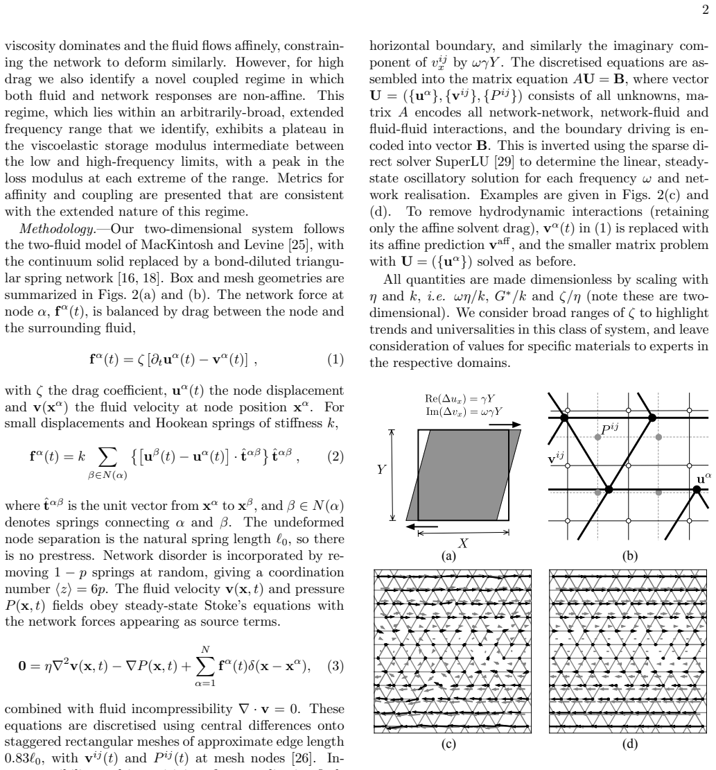
The machinery is a matrix-based solver for the linear oscillatory response of a bond-diluted triangular spring network coupled to a viscous solvent through point drag forces at network nodes: each node obeys f_α = ζ(∂_t u_α − v_α), and the fluid satisfies Stokes' equations with the nodal forces as delta-function sources. The coupled equations are discretized on staggered meshes and solved as one sparse matrix equation for the complex amplitudes of displacements, fluid velocities, and pressures under oscillatory shear. Three dimensionless metrics quantify non-affinity of the network, non-affinity of the fluid, and decoupling between the two, and the complex modulus is fit to a parallel spring plus two Maxwell units to extract the plateau's characteristic rates.
What would settle it
Replace the nodal point drag in the same coupled equations with a drag distributed continuously along each spring segment (for instance by discretizing each fiber into beads that all experience solvent drag), and compute the complex modulus across ωη/k ≪ 1 ≪ ωζ/k; if the intermediate plateau and its twin loss peaks vanish, the central claim is false. A bulk rheology experiment on a well-characterized immersed fiber network with independently known ζ/η would also test it: the predicted plateau and two loss peaks must appear between the low- and high-frequency limits.
Extended reading notes
Core claim
The central discovery is that a fluid-immersed, disordered spring network can store elastic energy in an intermediate-frequency regime in which neither the network displacement field nor the fluid velocity field is affine, while the two fields remain strongly coupled. For drag coefficient ζ much larger than the solvent viscosity η and for frequencies satisfying ωη/k ≪ 1 ≪ ωζ/k, the storage modulus G′(ω) flattens into a plateau G_NA lying between the low-frequency modulus G0 and the high-frequency affine modulus G_aff = pk√3/4, and the network contribution to G″(ω) shows two peaks at the plateau edges. The plateau is absent when hydrodynamic interactions are removed by replacing the true fluid velocity with its affine prediction. Fitting the spectra to a spring plus two viscoelastic Maxwell elements gives effective rates ζeff ≈ ζ and ηeff ≈ η, and the plateau value scales linearly with p − p∗ in a way that cannot be mapped onto G0 by changing network density.
Load-bearing premise
The load-bearing premise is that the fluid–network interaction can be represented entirely as point drag forces acting at the discrete network nodes; if realistic coupling along the full length of each fiber changes the physics, the intermediate plateau may disappear.
Editorial extensions
If this is right
- For p > p_c, strong drag produces an intermediate plateau G_NA in the storage modulus, bracketed by two peaks in the network contribution to the loss modulus.
- The plateau disappears if hydrodynamic interactions are switched off, so any experiment that sees it is direct evidence of full fluid–network coupling.
- The fitted plateau frequencies scale with the bare parameters, ζeff ≈ ζ and ηeff ≈ η, so the plateau location is set by the same drag and viscosity that define the regimes.
- Below the rigidity threshold, any finite frequency gives terminal scaling G′ ∼ ω² and G″ ∼ ω, meaning the solvent rigidifies floppy networks at all accessible frequencies.
- Network configurations in the intermediate plateau deform differently from vacuum non-affinity at the same modulus, so tuning p cannot reproduce the plateau by rescaling a vacuum network.
Reading between the lines
- If node-only drag is replaced by distributed drag along fiber segments, the plateau may persist with only rescaled relaxation rates; a clean way to check is a bead-spring or immersed-boundary simulation where the fluid force is applied along the whole spring, not just at endpoints.
- The plateau's high and low edges are set by η and ζ separately, so varying solvent viscosity at fixed network density should shift only one edge; measuring that would show whether the two-Maxwell description is physically meaningful.
- The paper's finite-frequency rigidification of sub-isostatic networks suggests that many 'soft' fiber materials may appear rigid in practice, with the fluid-controlled plateau providing a second stiffness scale that cells or other sensors could in principle detect.
Signed reviews
Editorial analysis
A structured set of objections, weighed in public.
Referee Report
Summary. The manuscript describes a matrix-based numerical solver for the linear oscillatory rheology of two-dimensional disordered spring networks immersed in a Stokes fluid, with network–fluid coupling through point drag at the nodes. The authors scan the drag coefficient ζ, fluid viscosity η, and frequency ω and identify four response regimes from affinity and coupling metrics. Their main claim is a previously unreported intermediate regime at ζ≫η in which both the fluid and the network respond non-affinely and remain coupled, producing an additional storage-modulus plateau G_NA between the low-frequency G_0 and the high-frequency affine G_aff, with two peaks in the network contribution to the loss modulus at the plateau boundaries. They also report linear dependence of the plateau moduli on bond density p and note that finite-frequency driving rigidifies sub-isostatic networks. The central results are presented as averaged spectra over ten 100×100 networks, supplemented by checks of mesh insensitivity and incompressibility.
Significance. If correct, the claimed fluid-coupled non-affine plateau would be a genuinely new element in the rheology of immersed fiber networks, distinct from the vacuum response and from one-way coupled models; it is also potentially relevant to biopolymer networks and hydrogels. The systematic parameter scan and the matrix-based solver are useful technical contributions, and the authors are careful to check mesh insensitivity and incompressibility and to average over multiple realizations. The significance, however, cannot be fully assessed from the manuscript as written: the stress formula in Eq. (4) is questionable, and the plateau characterization relies on a Maxwell-mode fit without error bars or residuals. These issues must be resolved before the new regime can be considered established.
major comments (3)
- [Viscoelastic spectra, Eq. (4)] The stress formula in Eq. (4) uses f_αβ ≡ f_β − f_α, the difference of the total nodal forces, rather than the force carried by the bond αβ. The standard pair virial for a central-force network requires F_αβ = k[(u_β − u_α)·t̂]t̂ contracted with (x_β − x_α). As written, Eq. (4) fails even in a uniformly strained one-dimensional chain, where interior nodes have f_α = 0 and the expression returns zero while every bond carries a nonzero force. Since all plateau and loss-peak claims are read from G*(ω) computed by this formula, this is a load-bearing issue. If the code uses the correct bond-force virial, Eq. (4) and the definition of f_αβ must be corrected; if the code implements Eq. (4) as written, the reported spectra do not measure the shear modulus.
- [Viscoelastic spectra, Eqs. (5)–(6) and Fig. 4] The identification of the intermediate plateau and the two loss peaks is obtained by fitting G′ and G″ to a two-Maxwell-unit ansatz whose two relaxation rates are by construction the fitted parameters. No error bars are shown for the modulus curves and no fit residuals are reported, and the finding ζ_eff≈ζ and η_eff≈η is therefore a consistency check built into the fit form rather than independent evidence. Please report per-frequency standard errors (the text says each curve is an average over 10 networks), the fit residuals, and a model-independent plateau criterion, such as the frequency range over which d log G′/d log ω stays within a small tolerance of zero and over which two resolved maxima in G″−ωη are visible.
- [Response regimes and Fig. 3] The new regime is identified from smooth crossovers in the metrics, and the scaling argument in the text explicitly stops short of predicting it: the text states that 'no terms in (3) dominate, so a limiting solution for v cannot be inferred' and that 'Fig. 3 suggests a smooth crossover'. To support the claim that this is a distinct regime rather than a crossover, please provide an independent diagnostic of the regime boundaries, for example a collapse of Γ_net, Γ_fl, and Γ_dc on ωζ/k and ωη/k, or a direct demonstration that the plateau width scales as ζ/η. Such a test would tie the plateau in G*(ω) to the regime identified from the metrics without relying on the fitted Maxwell modes.
minor comments (5)
- [Fig. 4] The axis labels in Fig. 4 are garbled: '10 3' should be '10^{-3}', and '(G′′ i ) / k' should be '(G′′ − ωη)/k' or similar.
- [Reference [28]] The name 'Tildesley' is misspelled as 'Tildedsley'.
- [Fig. 5] Fig. 5 shows no error bars for G_NA, G_0, or Γ_net even though each data point is an average over 10 networks; the uncertainties on the fitted p* values are given, but the underlying scatter should be visible.
- [Supplemental Material] The Supplemental Material (Figs. S1–S4) is cited but was not included with the manuscript; it should be submitted for review because the mesh-insensitivity and incompressibility checks and the p<p_c spectra are used to support claims in the main text.
- [Methodology] In the Methodology paragraph, 'The fluid velocity vα(t) at mesh nodes' should read 'at network nodes', since the staggered mesh refers to the fluid grid points.
Circularity Check
No significant circularity: the coupled non-affine plateau is read directly from the simulated G*(ω) spectra, and the Maxwell fits are post-hoc characterization, not fitted inputs renamed as predictions.
full rationale
The paper's central claim is a numerical observation from a self-contained linear solve of the coupled Stokes/spring equations (Eqs. 1-3), so it does not reduce to its inputs by construction. The plateau in G'(ω) is identified in the raw data before any fitting: "For p>p_c, a plateau emerges in G′(ω) as ζ→∞" (Viscoelastic spectra section), with the two-Maxwell form of Eqs. (5)-(6) used only afterward to extract GNA and the crossover rates. Thus the plateau is not imposed by the fit. The fitted rates ζeff≈ζ and ηeff≈η are consistency checks, not constructed identities: the rates are free fit parameters, and their agreement with the physical drag/viscosity scales is nontrivial supporting evidence. The affinity metrics Γnet, Γfl, Γdc are independent observables computed from the same solved fields; their agreement with the modulus-based regime picture is a finding, not an equivalence. Self-citations (e.g., [14], [15], [32]) are used for model context or prior validation, not as a load-bearing uniqueness theorem or an ansatz smuggled in by citation. The Discussion's acknowledged limitation that coupling only at nodes is "numerically convenient" and generalization "desirable" is a modeling-validity caveat, not circularity. A separate correctness concern exists: Eq. (4) defines f_αβ = f_β − f_α, the difference of total node forces, rather than the bond force, which is not the standard virial stress; this is a potential numerical-validity issue, not a circularity, and does not affect the circularity score.
Assumptions & free parameters
free parameters (4)
- effective drag rate zeta_eff/k =
approx zeta/k
- effective viscosity rate eta_eff/k =
approx eta/k
- p* for G_NA(p) linear fit =
0.406(2)
- p* for G_0(p) linear fit =
0.6698(4)
assumptions (4)
- domain assumption Steady-state Stokes equations with point forces describe the fluid, Eq. (3).
- domain assumption Athermal network with Hookean springs and no prestress, Eq. (2), represents a fiber network.
- domain assumption Oscillatory steady state and linear response are valid.
- domain assumption Two-dimensional bond-diluted triangular lattice is representative of 3D network behavior.
Cite this review
Pith. "Pith review of Non-affinity and fluid-coupled viscoelastic plateau for immersed fiber networks." pith.science (2026). https://pith.science/paper/3PW4HG4Z
@misc{pith2026190807768,
  author       = {Pith},
  title        = {Pith review of: Non-affinity and fluid-coupled viscoelastic plateau for immersed fiber networks},
  year         = {2026},
  howpublished = {\url{https://pith.science/paper/3PW4HG4Z}},
  note         = {Machine review of arXiv:1908.07768}
}
read the original abstract
We employ a matrix-based solver for the linear rheology of fluid-immersed disordered spring networks to reveal four distinct dynamic response regimes. One regime - completely absent in the known vacuum response - exhibits coupled fluid flow and network deformation, with both components responding non-affinely. This regime contains an additional plateau (peak) in the frequency-dependent storage (loss) modulus - features which vanish without full hydrodynamic interactions. The mechanical response of immersed networks such as biopolymers and hydrogels is thus richer than previously established, and offers additional modalities for design and control through fluid interactions.
Figures


Figures from the paper (2 more)


Reference graph
Works this paper leans on
-
[1]
Bray, Cell movements (Garland, New York, 2001)
D. Bray, Cell movements (Garland, New York, 2001)
work page 2001
-
[2]
J. A. Burdick and R. L. Mauck, Biomaterials for Tissue Engineering Applications (Springer, Vienna, 2011)
work page 2011
-
[3]
G. K. Batchelor, An Introduction to Fluid Dynamics (Cambridge University Press, Cambridge, 1967)
work page 1967
-
[4]
Doi and S
M. Doi and S. F. Edwards, The Theory of Polymer Dy- namics (Oxford University Press, Oxford, 1986)
1986
-
[5]
Rubinstein and R
M. Rubinstein and R. H. Colby,Polymer Physics (Oxford University Press, Oxford, 2003)
2003
-
[6]
Chaikin, in Soft Fragile Matter, edited by M
P. Chaikin, in Soft Fragile Matter, edited by M. E. Cates and M. R. Evans (Institute of Physics, Bristol, 1999) pp. 315–348
work page 1999
- [7]
-
[8]
J. L. McWhirter, H. Noguchi, and G. Gompper, Proc. Natl. Acad. Sci. 106, 6039 (2009)
work page 2009
Show all 37 references
-
[9]
Alava and K
M. Alava and K. Niskanen, Reports Prog. Phys. 69, 669 (2006)
2006
-
[10]
C. P. Broedersz, X. Mao, T. C. Lubensky, and F. C. Mackintosh, Nat. Phys. 7, 983 (2011)
2011
-
[11]
C. Tang, R. V. Ulijn, and A. Saiani, Langmuir 27, 14438 (2011)
2011
-
[12]
Hoffmann, K
T. Hoffmann, K. M. Tych, M. L. Hughes, D. J. Brock- well, and L. Dougan, Phys. Chem. Chem. Phys. 15, 15767 (2013)
2013
-
[13]
H. Li, N. Kong, B. Laver, and J. Liu, Small 12, 973 (2016)
2016
-
[14]
L. G. Rizzi, S. Auer, and D. A. Head, Soft Matter 12, 4332 (2016)
2016
-
[15]
E. M. Huisman, C. Storm, and G. T. Barkema, Phys. Rev. E - Stat. Nonlinear, Soft Matter Phys. 82, 061902 (2010)
2010
-
[16]
M. G. Yucht, M. Sheinman, and C. P. Broedersz, Soft Matter 9, 7000 (2013)
2013
-
[17]
H. E. Amuasi, A. Fischer, A. Zippelius, and C. Heussinger, J. Chem. Phys. 149, 084902 (2018)
2018
-
[18]
Dennison and H
M. Dennison and H. Stark, Phys. Rev. E 93, 022605 (2016)
2016
-
[19]
H. C. De Cagny, B. E. Vos, M. Vahabi, N. A. Kurni- awan, M. Doi, G. H. Koenderink, F. C. MacKintosh, and D. Bonn, Phys. Rev. Lett. 117, 217802 (2016)
2016
-
[20]
Vahabi, B
M. Vahabi, B. E. Vos, H. C. G. D. Cagny, D. Bonn, G. H. Koenderink, and F. C. Mackintosh, Phys. Rev. E 97, 032418 (2018)
2018
-
[21]
B. et al.. Trappmann, Nature Materials 11, 642 (2012)
2012
-
[22]
A. J. Engler, S. Sen, H. L. Sweeney, and D. E. Discher, Cell 125, 677 (2006)
2006
-
[23]
Chaudhuri, L
O. Chaudhuri, L. Gu, M. Darnell, D. Klumpers, S. A. Bencherif, J. C. Weaver, N. Huebsch, and D. J. Mooney, Nature Comm. 6, 6365 (2015)
2015
-
[24]
O. e. a. Chaudhuri, Nature Materials 15, 326 (2016)
2016
-
[25]
F. C. Mackintosh and A. J. Levine, Phys. Rev. Lett. 100, 018104 (2008)
2008
-
[26]
J. D. Anderson, Computational fluid dynamics (McGraw- Hill, New York, 1995)
1995
-
[27]
See Supplemental Material at [URL will by inserted by publisher] for additional figures
-
[28]
M. P. Allen and D. J. Tildedsley, Computer Simulations of Liquids (Clarendon Press, Oxford, 1987)
1987
-
[29]
J. W. Demmel, S. C. Eisenstat, J. R. Gilbert, X. S. Li, and J. W. H. Liu, SIAM J. Matrix Anal. Appl. 20, 720 (1999)
1999
-
[30]
H. M. James and E. Guth, J. Chem. Phys.11, 455 (1943)
1943
-
[31]
H. A. Barnes, J. F. Hutton, and K. Walters, An Intro- duction to Rheology (Elsevier, Amsterdam, 1989)
1989
-
[32]
Dennison, M
M. Dennison, M. Sheinman, C. Storm, and F. C. Mack- intosh, Phys. Rev. Lett. 111, 095503 (2013)
2013
-
[33]
Sahimi, Heterogeneous Materials I: Linear Trans- port and Optical Properties (Springer-Verlag, New York, 2003)
M. Sahimi, Heterogeneous Materials I: Linear Trans- port and Optical Properties (Springer-Verlag, New York, 2003)
2003
-
[34]
J. M. van Doorn, L. Lageschaar, J. Sprakel, and J. van Der Gucht, Phys. Rev. E 95, 042503 (2017)
2017
-
[35]
M. F. Vermeulen, A. Bose, C. Storm, and W. G. Ellen- broek, Phys. Rev. E 96, 053003 (2017)
2017
-
[36]
Merkel, K
M. Merkel, K. Baumgarten, B. P. Tighe, and M. L. Manning, Proc. Natl. Acad. Sci. 116, 6560 (2019)
2019
-
[37]
du Roure, A
O. du Roure, A. Lindner, E. N. Nazockdast, and M. J. Shelley, Ann. Rev. Fluid Mech. 51, 539 (2019)
2019
Reviewed August 14, 2026 · model on record in the stance chip above.
Discussion (0). Continue with ORCID to comment.