REVIEW 2 major objections 4 minor 46 references
`Regression Anytime' with Brute-Force SVD Truncation
T0 review · 2 major / 4 minor · reviewed 2026-08-14 · deepseek-v4-flash
Pith's one-line read A least-squares Monte Carlo algorithm that, under sufficient smoothness, estimates conditional expectations with Malliavin weights at any chosen polynomial convergence rate.
desk verdict A strong, genuinely useful LSMC paper whose central theorem is currently marred by a localized sign error in the written proof — repairable, but the theorem as printed is not proven. read the letter →
The pith
A machine-rendered reading of the paper's core claim, the machinery that carries it, and where it could break.
The reading
What carries the argument
The machinery has three parts. First, 'regression anytime' basis functions: products of an indicator of a cube in the $X_1$-space and Legendre polynomials of total degree at most $Q$ in the $X_2$-variable, rescaled to the cube. Because the $X_1$-factor is pulled out of the conditional expectation, the expectation of the basis times the Malliavin weight is available in closed form through moments of a truncated normal, so the estimator includes automatic differentiation. Second, importance sampling: the law of $X_1$ is reweighted to a stratified uniform distribution on a cube, so the expected regression matrix is nearly orthonormal and its extremal eigenvalues are bounded away from zero. Third, brute-force SVD truncation: for each empirical regression matrix, either the ordinary least-squares solution is kept when the smallest singular value is above the threshold $\tau L$, or all coefficients are set to zero, preventing variance explosions. The key estimate is Theorem 4.3, whose proof uses the matrix Bernstein inequality to show that the bad-event probability decays exponentially in the number of samples $L$, making the statistical error negligible relative to the polynomial approximation error.
What would settle it
Take the one-dimensional example of Section 3.1 but with unbounded coefficients, e.g. $X_2=X_1+\mu X_1\Delta+\sigma X_1\sqrt{\Delta}\xi$ (geometric Brownian motion), keep the same smooth $y$, and measure $\mathbb{E}\int|\hat z-z|^2\mu_1(dx)$ for $\rho=2$; if the observed rate is slower than $\Delta^2$ (up to log factors), the boundedness assumption is essential. Alternatively, in a bounded-coefficient example, compute the empirical probability that the smallest singular value falls below $\tau L$ as $L$ grows; if that probability does not decay exponentially, the matrix Bernstein bound behind Theorem 4.3 would need revision.
Extended reading notes
Core claim
The central claim is Theorem 2.5: fix a requested rate $\rho\in\mathbb{N}$; if $y\in C_b^{Q+1}(\mathbb{R}^D)$ with $Q\ge|\iota|_1+\rho$, then Algorithm 2.3 with the stated parameter choices produces an estimator $\hat z$ satisfying $\mathbb{E}\int |\mathbb{E}[H_{\iota,\Delta}(\xi)y(X_2)|X_1=x]-\hat z(x)|^2\mu_1(dx)\le C\log(\Delta^{-1})^{D/2}\Delta^\rho$ for all sufficiently small $\Delta$. Here $H_{\iota,\Delta}$ is a scaled multivariate Hermite weight, and $X_2$ is one Euler step starting from $X_1$. The engine behind the rate is Theorem 4.3: for a fixed basis, noiseless least-squares regression with brute-force SVD truncation has statistical error that decays exponentially in the number of samples, because the matrix Bernstein inequality controls the probability that the smallest singular value of the empirical regression matrix falls below its threshold. That exponential control is what lets the number of basis functions and the number of samples grow at the same rate, converting a smoothness assumption into a tunable polynomial convergence rate.
Load-bearing premise
The rate proof assumes the current state $X_1$ has a density dominated by a Gaussian density and that the drift and diffusion coefficients are bounded, so the state space can be safely truncated to a cube whose radius grows like $\sqrt{\log\Delta^{-1}}$; if that assumption fails, the truncation bias and the conditioning of the local regressions are no longer controlled.
Editorial extensions
If this is right
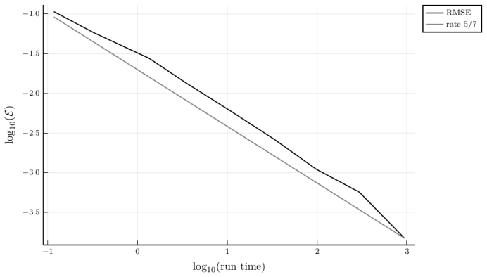
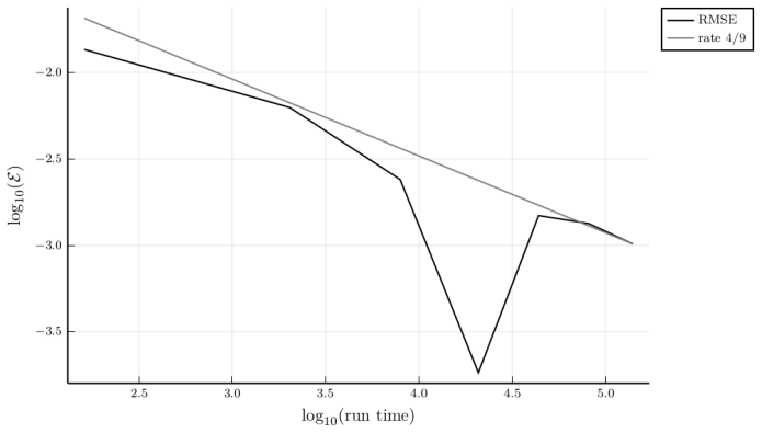
- For a fixed smoothness class, the user can choose $\rho$ and obtain mean squared error of order $\Delta^\rho$; in terms of computational complexity, achieving accuracy $\epsilon$ costs roughly $\epsilon^{-D/(Q+1)(1+|\iota|_1/\rho)}$, which is better than the $\epsilon^{-2}$ Monte Carlo baseline when the dimension-to-smoothness ratio is small.
- The estimator simultaneously approximates Malliavin derivatives of the regression function, so one run of the algorithm supplies derivative terms needed in backward recursions for nonlinear option pricing and BSDE solvers.
- In dynamic programming applications, each time step only requires one-step Euler samples; no full path simulation or path storage is needed, and per-cube regressions are independent, keeping memory use proportional to the number of coefficients rather than the number of trajectories.
- The SVD-truncation lemma (Theorem 4.3) applies to any bounded basis with controlled eigenvalues, so the convergence-rate mechanism is not tied to Legendre polynomials and can be reused with other basis families.
- The noiseless interpolation result matches, up to log factors, the optimal rates for interpolation with random design, giving a theoretical benchmark for regression-later-type algorithms beyond the specific RAWBFST setting.
Reading between the lines
- A natural testable extension is to weaken Assumption 2.1: for processes with unbounded coefficients such as geometric Brownian motion, the Gaussian-density and boundedness conditions fail; one could check numerically whether a growing truncation radius still yields a rate close to the stated polynomial rate or whether the rate degrades to a Monte Carlo rate.
- The paper's backward error propagation in the UVM and BSDE examples is heuristic rather than proven; if the one-step rate of Theorem 2.5 does not propagate through many nested conditional expectations, the practical speed-up in long-horizon problems would be smaller than the one-step analysis suggests.
- The brute-force SVD rule is binary: keep all coefficients or set all to zero. A natural alternative is a soft or partial truncation that keeps the largest singular values; the exponential tail bound suggests such a variant might retain the rate while reducing bias, but this is not explored in the paper.
- The noiseless regression analysis treats the design points as random samples; replacing them with a deterministic quasi-Monte Carlo sequence could remove the log factors and give exact polynomial rates, though the eigenvalue control would need to be re-established for that setting.
Signed reviews
Editorial analysis
A structured set of objections, weighed in public.
Referee Report
Summary. The paper proposes RAWBFST, a least-squares Monte Carlo algorithm for approximating conditional expectations of the form E[H_{ι,Δ}(ξ)y(X_2)|X_1], where X_2 is one Euler step and H_{ι,Δ} is a Malliavin-type weight. The algorithm combines a 'regression anytime' basis construction (local Legendre polynomials depending on both current and future states), stratified uniform sampling with importance weighting, and a brute-force SVD truncation of the empirical regression matrix. The central theoretical result, Theorem 2.5, claims that under a Gaussian-type density bound on the law of X_1 and bounded drift/diffusion coefficients, the L2 error can be made to decay as C log(Δ^{-1})^{D/2} Δ^ρ for any prescribed ρ∈N, provided y is smooth enough. Section 4 develops a standalone noiseless interpolation theorem with exponential statistical error via the matrix Bernstein inequality, and Section 5 gives the proof of Theorem 2.5. Numerical experiments cover a second-derivative approximation, an uncertain volatility model, and a five-dimensional BSDE.
Significance. If the main theorem is correct, this is a substantial contribution to least-squares Monte Carlo: it provides a generic estimator whose convergence rate can be tuned to any polynomial order by increasing smoothness, with explicit parameter choices that are prescribed rather than calibrated to the target result. Theorem 4.3, an exponential concentration bound for noiseless SVD-truncated least squares with non-orthonormal bases, is a useful building block in its own right. The numerical experiments are carefully reported and support the theoretical rates. The main limitations are the assumption of bounded coefficients and Gaussian-type densities (which excludes, for example, geometric Brownian motion) and the fact that the backward dynamic programming applications in Sections 3.2 and 3.3 are exploratory: their error propagation through time steps is heuristic rather than proved.
major comments (2)
- [Section 5, proof of Theorem 2.5, display after Lemma 5.2 and Eq. (29)] Lemma 5.2 is applied with Γ̃_i = {s_{i,K}^2 ≥ τL}, so its probability term is max_i P(Γ̃_i^c) = max_i P(s_{i,K}^2 < τL). The proof instead writes max_i P(s_{i,K}^2 ≥ τL) and then states in (29) that this quantity is O(Δ^ρ). This is not true: by Lemma 5.3, λ_min(R_Δ)→1, and the empirical Gram matrix concentrates, so s_{i,K}^2/L → 1 in probability as Δ→0; for the fixed τ<1, the event {s_{i,K}^2 ≥ τL} therefore has probability tending to 1, not O(Δ^ρ). Lemma 4.7, inequality (19), and Lemma 5.5 only bound the complementary event {s_{i,K}^2 < τL}. The fix is a sign change in two places: replace ≥ with < in the probability term after Lemma 5.2 and in the first line of (29). The expectation term in (29), which uses 1_{s_{i,K}^2 ≥ τL}, is correct, so with this correction the proof becomes coherent.
- [Section 5, proof of Theorem 2.5, Taylor remainder estimate] After bounding inf_α E|y − Σ α_k η_k|^2 by C_4^2 E[|X_2^{Δ,r2,i} − a_i|_2^{2(Q+1)}], the proof states that the term E[|X_2^{Δ,r2,i} − a_i|_2^{2(|ι|_1+ρ+1)}] is of order Δ^{(2Q+2)γ_cube} = Δ^{ρ+|ι|_1}. The exponent must be 2(Q+1), not 2(|ι|_1+ρ+1), to match the Taylor remainder of degree Q; the displayed equality to Δ^{ρ+|ι|_1} is correct only when Q = |ι|_1+ρ. For the general case Q ≥ |ι|_1+ρ allowed by Theorem 2.5, the written exponent gives a different, generally larger bound. This is a localized error, but it appears in the proof of the main theorem and should be corrected.
minor comments (4)
- [Remark 2.4, moment recursion] The recursion for m_{q,r} = E[[ξ_1]^q_r] appears to have an incorrect initial value: for the censored normal variable [ξ]_r, m_{0,r} should be 1, not 0. With m_{0,r}=0, the formula gives m_{2,r} negative for small r. Please also check the factor multiplying (1−Φ(r)); a direct integration by parts for the two-sided censored moment gives a factor 2 in the boundary term.
- [Lemma 5.3, lower bound for m_Δ] The assertion that (1,...,1) ∈ supp(X^(2)) is not literally true when b ≠ 0, because the support is the cube [-1,1]^D shifted by an O(Δ^{1−γ_cube}) vector. The stated limit is still correct by continuity of the Legendre polynomials and convergence of the support in Hausdorff distance; please rephrase the argument.
- [Sections 3.2 and 3.3, dynamic programming heuristic] The backward recursion applications assume, without proof, that the one-step error bound of Theorem 2.5 propagates through many time steps at the stated rate. The text already labels these sections exploratory, but it would be helpful to state explicitly in the conclusions that no rigorous error bound for the full backward recursion is proved in this paper.
- [Throughout, notation] Equation (4) would benefit from parentheses around the exponent of ε; the intended expression is ε^{-D/(Q+1) (1+|ι|_1/ρ)}. The current line breaks make the exponent structure ambiguous.
Circularity Check
No significant circularity: the rate in Theorem 2.5 is derived from explicit parameter choices and external concentration inequalities; the only self-referential element is the motivational 'regression anytime' framing from the authors' earlier work.
full rationale
Walking the derivation chain, the central claim (Theorem 2.5) is obtained by decomposing the mean-squared error into four parts: Gaussian-innovation truncation (Lemma 5.1), change of measure and removal of the Malliavin weight (Lemma 5.2), statistical error of noiseless SVD-truncated regression (Theorem 4.3, Lemmas 4.7 and 5.5), and local Taylor approximation. Each parameter in Theorem 2.5 is prescribed rather than fitted: gamma_cube is set so the Taylor remainder is Delta^{rho+|iota|_1}; gamma_{1,trunc}=rho and gamma_{2,trunc}=1.5(|iota|_1+rho) make the truncation terms Delta^rho; L grows logarithmically so the matrix-Bernstein tail in Lemma 5.5 is Delta^rho; and tau is constrained by the explicit constant c*_paths. No constant is calibrated to the target rate, and no lemma assumes the conclusion. The 'regression anytime' idea is acknowledged as a re-framing of 'regression later' rather than a new algorithm, and citations to the authors' earlier work ([6], [7], [8], [31]) are contextual or motivational, not used to justify the rate proof; Theorem 4.3 is proved in the paper from Tropp's matrix Bernstein inequality [44]. The exploratory numerical sections explicitly state heuristic assumptions rather than deriving predictions from Theorem 2.5 (Section 3.2: 'we here assume that the same is true for RAWBFST in the non-linear case'; Section 3.3: 'Calibrating the algorithm to an error of the order Delta^{1/2} ... heuristically'). The proof of Theorem 2.5 contains a localized sign/event mismatch in the application of Lemma 5.2 (it bounds P(s_{i,K}^2 >= tau L) where Lemma 5.2 requires P(s_{i,K}^2 < tau L), and (29) states the former is O(Delta^rho)); this is a correctness flaw, not a circularity, because the lemmas supply the complementary-event bound and the argument is repairable by a sign correction. Overall, the derivation is self-contained and Section 3.1 benchmarks it against closed-form solutions, so there is no load-bearing circular step.
Assumptions & free parameters
free parameters (3)
- tau =
0.0233 in numerical illustrations
- c1,paths =
1.1 c*_paths(Q,D) in examples
- sigma0^2 =
0.1 T in UVM and 5D BSDE examples
assumptions (6)
- standard math Matrix Bernstein inequality (Tropp 2012, Theorem 4.8) for sums of independent zero-mean random matrices.
- standard math Gershgorin's theorem and the eigenvalue perturbation bound |lambda_min(Sigma1) - lambda_min(Sigma2)| <= ||Sigma1 - Sigma2||_2.
- standard math Orthonormality of scaled Legendre polynomials on [-1,1] with respect to the Lebesgue measure.
- domain assumption Assumption 2.1: the law of X1 has a density with Gaussian upper bound and the coefficients b, sigma are bounded.
- domain assumption Smoothness hypothesis y in C_b^{Q+1}(R^D) with Q >= |iota|1 + rho in Theorem 2.5.
- domain assumption One-step Euler scheme structure X2 = X1 + b(X1)Delta + sigma(X1) sqrt(Delta) xi with independent standard Gaussian xi.
Cite this review
Pith. "Pith review of `Regression Anytime' with Brute-Force SVD Truncation." pith.science (2026). https://pith.science/paper/3QBULZII
@misc{pith2026190808264,
  author       = {Pith},
  title        = {Pith review of: `Regression Anytime' with Brute-Force SVD Truncation},
  year         = {2026},
  howpublished = {\url{https://pith.science/paper/3QBULZII}},
  note         = {Machine review of arXiv:1908.08264}
}
read the original abstract
We propose a new least-squares Monte Carlo algorithm for the approximation of conditional expectations in the presence of stochastic derivative weights. The algorithm can serve as a building block for solving dynamic programming equations, which arise, e.g., in non-linear option pricing problems or in probabilistic discretization schemes for fully non-linear parabolic partial differential equations. Our algorithm can be generically applied when the underlying dynamics stem from an Euler approximation to a stochastic differential equation. A built-in variance reduction ensures that the convergence in the number of samples to the true regression function takes place at an arbitrarily fast polynomial rate, if the problem under consideration is smooth enough.
Figures


Figures from the paper (2 more)

Reference graph
Works this paper leans on
-
[1]
(2013) Reducing variance in the numerical solution of BSDEs
Alanko, S., Avellaneda, M. (2013) Reducing variance in the numerical solution of BSDEs. C. R. Math. Acad. Sci. Paris 351 135–138
work page 2013
-
[2]
(2004) Primal-dual simulation algorithm for pricing multi- dimensional American options
Andersen, L., Broadie, M. (2004) Primal-dual simulation algorithm for pricing multi- dimensional American options. Manage. Sci. 50 1222–1234
work page 2004
-
[3]
(1995) Pricing and hedging derivative securities in markets with uncertain volatilities
Avellaneda, M., Levy, A., Par´ as, A. (1995) Pricing and hedging derivative securities in markets with uncertain volatilities. Appl. Math. Finance , 2 73–88
work page 1995
-
[4]
Regress-Later Monte Carlo for optimal control of Markov processes
Balata, A., Palczewski, J. (2018) Regress-later Monte Carlo for optimal control of Markov processes. arXiv:1712.09705
work page Pith review arXiv 2018
-
[5]
(2017) Nonparametric estimation of a function from noiseless observations at random points
Bauer, B., Devroye, L., Kohler, M., Krzyzak, A., Walk, H. (2017) Nonparametric estimation of a function from noiseless observations at random points. J. Multivariate Anal. 160 93–104
work page 2017
-
[6]
(2017) Iterative improvement of lower and upper bounds for backward SDEs
Bender, C., G ¨artner, C., Schweizer, N. (2017) Iterative improvement of lower and upper bounds for backward SDEs. SIAM J. Sci. Comput. 39 B442–B466
work page 2017
-
[7]
(2018) Pathwise dynamic programming
Bender, C., G ¨artner, C., Schweizer, N. (2018) Pathwise dynamic programming. Math. Oper. Res., 43 965–995
work page 2018
-
[8]
(2012) Least squares Monte Carlo for BSDEs
Bender, C., Steiner, J. (2012) Least squares Monte Carlo for BSDEs. In: Carmona, R. et al. (eds.) Numerical Methods in Finance , Springer, Berlin, pp. 257–289
work page 2012
Show all 46 references
-
[9]
(2013) Preliminary control variates to improve empirical regression methods
Ben Zineb, T., Gobet, E. (2013) Preliminary control variates to improve empirical regression methods. Monte Carlo Methods Appl. , 19, 331–354
2013
-
[10]
(2013) Fast convergence of regress-later esti- mates in least squares Monte Carlo
Beutner, E., Schweizer, J., Pelsser, A. (2013) Fast convergence of regress-later esti- mates in least squares Monte Carlo. arXiv:1309.5274
2013 arXiv
-
[11]
(2004) Discrete-time approximation and Monte Carlo simula- tion of backward stochastic differential equations.Stochastic Process
Bouchard, B, Touzi, N. (2004) Discrete-time approximation and Monte Carlo simula- tion of backward stochastic differential equations.Stochastic Process. Appl.111 175–206
2004
-
[12]
W., Goyal, A., Santa-Clara, P., Stroud, J
Brandt, M. W., Goyal, A., Santa-Clara, P., Stroud, J. R. (2005) A simulation ap- proach to dynamic portfolio choice with an application to learning about return pre- dictability. Rev. Financ. Stud. 18 831–873
2005
-
[13]
Chau, K. W. , Oosterlee C. W. (2019) Stochastic grid bundling method for backward stochastic differential equations. Int. J. Comput. Math. 96 2272–2301
2019
-
[14]
A., Leviatan, D
Cohen, A., Davenport, M. A., Leviatan, D. (2013) On the stability and accuracy of least squares approximations. Found. Comput. Math. 13 819–834
2013
-
[15]
(2017) Optimal weighted least-squares methods
Cohen, A., Migliorati, G. (2017) Optimal weighted least-squares methods. SMAI J. Comput. Math. 3 181–203. 39
2017
-
[16]
G., Stentoft, L
Denault, M., Simonato, J. G., Stentoft, L. (2013) A simulation-and-regression ap- proach for stochastic dynamic programs with endogenous state variables.Comput. Oper. Res. 40 2760–2769
2013
-
[17]
(2011) A probabilistic numerical method for fully nonlinear parabolic PDEs
Fahim, A., Touzi, N., Warin, X. (2011) A probabilistic numerical method for fully nonlinear parabolic PDEs. Ann. Appl. Probab. 21 1322–1364
2011
-
[18]
(2004) Monte Carlo Methods in Financial Engineering
Glasserman, P. (2004) Monte Carlo Methods in Financial Engineering. Springer, New York
2004
-
[19]
(2004) Simulation for American options: Regression now or regression later? In: Niederreiter, H
Glasserman, P., Yu, B. (2004) Simulation for American options: Regression now or regression later? In: Niederreiter, H. (ed.) Monte Carlo and Quasi-Monte Carlo Methods 2002, Springer, Berlin, pp. 213–226
2004
-
[20]
(2007) Error expansion for the discretization of backward stochastic differential equations
Gobet, E., Labart, C. (2007) Error expansion for the discretization of backward stochastic differential equations. Stochastic Process. Appl. 117 803–829
2007
-
[21]
G., Turkedjiev, P., V´ azquez, C
Gobet, E., L´ opez-Salas, J. G., Turkedjiev, P., V´ azquez, C. (2016) Stratified regression Monte-Carlo scheme for semilinear PDEs and BSDEs with large scale parallelization on GPUs. SIAM J. Sci. Comput. 38 C652–C677
2016
-
[22]
H., van Loan, C
Golub, G. H., van Loan, C. H. (1996) Matrix Computations. 3rd edition, Johns Hop- kins University Press, Baltimore
1996
-
[23]
(2011) The uncertain volatility model: a Monte Carlo approach
Guyon, J., Henry-Labord` ere, P. (2011) The uncertain volatility model: a Monte Carlo approach. J. Comput. Finance 14 37–71
2011
-
[24]
(2002) A Distribution-Free Theory of Nonparametric Regression
Gy ¨orfi, L., Kohler, M., Krzyzak, A., Walk, H. (2002) A Distribution-Free Theory of Nonparametric Regression. Springer, New York
2002
-
[25]
Hansen, P. C. (1987) The truncated SVD as a method for regularization. BIT 27 534–553
1987
-
[26]
A., Johnson, C
Horn, R. A., Johnson, C. R. (1990) Matrix Analysis . Cambridge University Press, Cambridge
1990
-
[27]
(2010) Inequalities for quantiles of the chi-square distribution
Inglot, T. (2010) Inequalities for quantiles of the chi-square distribution. Probab. Math. Statist. 30 339–351
2010
-
[28]
Jain, S., Oosterlee, C. W. (2015) The stochastic grid bundling method: efficient pricing of Bermudan options and their Greeks. Appl. Math. Comput. 269 412–431
2015
-
[29]
(2014) A numerical algorithm for fully non- linear HJB equations: An approach by control randomization
Kharroubi, I., Langren´ e, N., Pham, H. (2014) A numerical algorithm for fully non- linear HJB equations: An approach by control randomization. Monte Carlo Methods Appl. 20 145–165
2014
-
[30]
(2013) Optimal global rates of convergence for interpolation problems with random design
Kohler, M., Krzyzak, A. (2013) Optimal global rates of convergence for interpolation problems with random design. Stat. Probab. Lett. 83 1871–1879
2013
-
[31]
(2020) Robust mul- tiple stopping – a pathwise duality approach
Laeven, R.J.A, Schoenmakers, J.G.M, Schweizer, N., Stadje, M. (2020) Robust mul- tiple stopping – a pathwise duality approach. arXiv:2006.01802
2020 arXiv
-
[32]
(2010) On some non asymptotic bounds for the Euler scheme
Lemaire, V., Menozzi, S. (2010) On some non asymptotic bounds for the Euler scheme. Electr. J. Probab. 15 1645–1681. 40
2010
-
[33]
(2006) Rate of convergence of an empirical regres- sion method for solving generalized backward stochastic differential equations,Bernoulli 12 889–916
Lemor, J.-P., Gobet, E., Warin, X. (2006) Rate of convergence of an empirical regres- sion method for solving generalized backward stochastic differential equations,Bernoulli 12 889–916
2006
-
[34]
A., Schwartz, E
Longstaff, F. A., Schwartz, E. S. (2001) Valuing American options by simulation: A simple least-squares approach. Rev. Financ. Stud. 14 113–147
2001
-
[35]
Lyons, T. J. (1995) Uncertain volatility and the risk-free synthesis of derivatives. Appl. Math. Finance 2 117–133
1995
-
[36]
S., Restrepo, M., Henderson, S
Maxwell, M. S., Restrepo, M., Henderson, S. G., Topaloglu, H. (2010) Approximate dynamic programming for ambulance redeployment.INFORMS J. Comput. 22 266–281
2010
-
[37]
(2017) Comparison of least squares Monte Carlo methods with applications to energy real options
Nadarajah, S., Margot, F., Secomandi, N. (2017) Comparison of least squares Monte Carlo methods with applications to energy real options. Eur. J. Oper. Res. 256 196–204
2017
-
[38]
(2016) The difference between LSMC and replicating port- folio in insurance liability modeling
Pelsser, A., Schweizer, J. (2016) The difference between LSMC and replicating port- folio in insurance liability modeling. Eur. Actuar. J. 6 441–494
2016
-
[39]
Powell, W. B. (2007) Approximate Dynamic Programming: Solving the curses of dimensionality. John Wiley & Sons, Hoboken
2007
-
[40]
(2018) Dynamic Programming
Rust, J. (2018) Dynamic Programming. In: Macmillan Publishers (eds.) The New Palgrave Dictionary of Economics , Palgrave Macmillan, London
2018
-
[41]
Schwartz, E. S. (2004) Patents and R&D as real options. Econ. Notes 33 23–54
2004
-
[42]
(2014) Discrete-time probabilistic approximation of path-dependent stochas- tic control problems, Ann
Tan, X. (2014) Discrete-time probabilistic approximation of path-dependent stochas- tic control problems, Ann. Appl. Probab. 24 1803–1834
2014
-
[43]
N., Van Roy, B
Tsitsiklis, J. N., Van Roy, B. (2001) Regression methods for pricing complex American-style options. IEEE Trans. Neural Networks 12 694–703
2001
-
[44]
Tropp, J. A. (2012) User-friendly tail bounds for sums of random matrices. Found. Comput. Math. 12 389–434
2012
-
[45]
Vanden, J. M. (2006) Exact superreplication strategies for a class of derivative assets. Appl. Math. Finance 13 61–87
2006
-
[46]
(2004) A numerical scheme for BSDEs
Zhang, J. (2004) A numerical scheme for BSDEs. Ann. Appl. Probab. 14 459–488. 41
2004
Reviewed August 14, 2026 · model on record in the stance chip above.
Discussion (0). Continue with ORCID to comment.