REVIEW 3 major objections 6 minor 2 cited by
Why Machine Learning Models Systematically Underestimate Extreme Values
T0 review · 3 major / 6 minor · reviewed 2026-08-11 · deepseek-v4-flash
Pith's one-line read Measurement noise in input features alone compresses machine-learning predictions toward the mean, no matter how much training data is used.
desk verdict A solid linear-regression treatment of attenuation bias for astronomy, embedded in a title that overclaims to all ML; worth refereeing with revision. read the letter →
The pith
A machine-rendered reading of the paper's core claim, the machinery that carries it, and where it could break.
The reading
What carries the argument
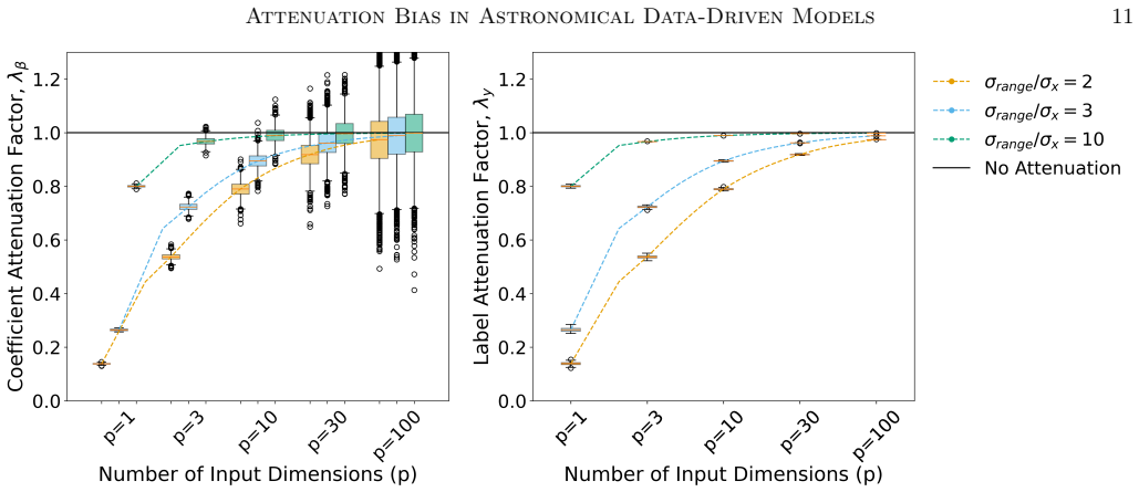
The load-bearing object is the attenuation factor λ = 1/(1+(σ_x/σ_range)^2), derived from the ordinary least squares expectation E[β̂] = Cov(x_obs,y_obs)/Var(x_obs). Input noise inflates the denominator without changing the numerator, so every coefficient is shrunk toward zero by the same ratio, and the predicted label is multiplied by λ. The multivariate extensions use the same decomposition: independent features give each coefficient its own λ_j, while perfectly correlated features produce a collective factor λ = (Σ a_j²)/(nσ_x²/S_x + Σ a_j²) that improves with dimensionality. For polynomial features the attenuation roughly scales as λ_n = 1/(1+n²(σ_x/σ_range)²), so higher-order terms suffer more severely.
What would settle it
Train any nonlinear regressor, such as a three-layer network, on synthetic data with known noise σ_x and measure the slope of predictions against true labels over a grid of σ_x/σ_range; if that slope does not follow λ = 1/(1+(σ_x/σ_range)^2), the paper's generalization to ML models fails, even though its linear result may stand.
Extended reading notes
Core claim
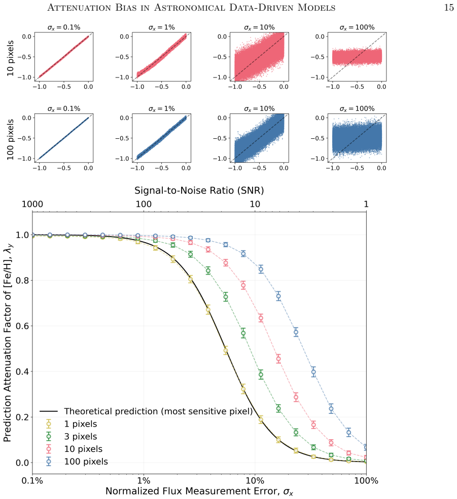
The central claim is that attenuation bias in direct spectra-to-label regression is a fundamental consequence of input measurement error, not of limited samples or imperfect labels. For univariate linear regression the expected slope is E[β̂] = λβ with λ = 1/(1+(σ_x/σ_range)^2), so predictions on new data are compressed by the same factor λ. The paper proves this bias is independent of training sample size and label noise, and shows it persists for independent multivariate features regardless of dimension. For perfectly correlated features the attenuation factor grows less severe with the number of features, approaching unity in the infinite-dimension limit, but real spectra fall short of that ideal because parameter variations such as temperature decorrelate features. Applied to APOGEE mock spectra, the framework predicts 1% bias under optimistic conditions and far larger biases at LAMOST/DESI-like resolutions and SNRs, with especially strong attenuation for elements that have few spectral features.
Load-bearing premise
The paper's broad title claims apply to all machine learning models, but its analytical proof covers linear regression; the step that generalizes to nonlinear networks is asserted, not derived.
Editorial extensions
If this is right
- More training data or more precise labels cannot fix the bias; only reducing input measurement uncertainty or exploiting feature correlations helps.
- In high-resolution, high-SNR spectroscopy (APOGEE-like), the bias is at the percent level, enough to matter for abundance and distance work; low-resolution surveys suffer much worse.
- Elements with few clean spectral features, such as oxygen, potassium, and vanadium, are especially affected because they cannot benefit from the correlated-feature mitigation.
- Discriminative models inherit input-noise bias, whereas generative models place the noise in the dependent variable and are therefore not attenuated by this mechanism.
- Power-law relations studied in log-log space, such as the M-σ relation or the Tully-Fisher relation, are vulnerable whenever dynamical-range-to-error ratios are O(1)-O(10).
Reading between the lines
- If the linear-regression result carries to nonlinear networks, then any error-ignorant discriminative model trained on noisy inputs will compress predicted labels even when its training loss is minimized; a direct test would compare the predicted-versus-true slope of a small neural network to λ across σ_x.
- The bias may explain part of the label-transfer discrepancies seen when stellar parameters are transferred between surveys; much of the residual in such catalogs could be modeled with the λ formula rather than treated as zero-point scatter.
- Because the bias is set by a ratio, co-adding or binning pixels (thereby reducing σ_x) would shrink attenuation even without changing the model, offering a cheaper mitigation than new instruments.
- The generative-versus-discriminative asymmetry suggests that hybrid approaches that fit spectra forward, or models that explicitly propagate input noise, will become necessary as surveys push to lower SNR.
Editorial analysis
A structured set of objections, weighed in public.
Referee Report
Summary. The paper derives and simulates attenuation (regression dilution) bias in linear regression with noisy input features. It obtains the formula \lambda = 1/(1+(\sigma_x/\sigma_{\rm range})^2) for the univariate case, extends the result to independent multivariate features, and gives an analytical result for perfectly correlated features under the assumptions x_{\rm true,j} = a_j x_{\rm true} and \beta = \beta a. It then applies the framework to synthetic APOGEE-like spectra, showing that even at R=24,000 and SNR=100 the predicted [Fe/H] is compressed by roughly one percent, with stronger effects at lower resolution or SNR. The final sections discuss implications for spectroscopy, distance measurements, and model choice, and argue that the insight extends beyond linear regression to machine learning generally.
Significance. If the linear-regression result is all that is claimed, the paper is a clean and useful contribution: the attenuation formula is derived from explicit assumptions rather than fitted, the simulations reproduce the formula across a wide range of \sigma_x/\sigma_{\rm range}, and the application to spectral inference gives a concrete quantitative warning. The correlated-feature case is also a helpful idealization, though its assumptions are narrow. The main value is as a reference for why linear spectral models compress labels. However, the paper's framing as a general statement about machine learning models is not supported by the evidence; the general claim is the part that would make the paper important beyond the linear case, and it currently rests on extrapolation. With the title and abstract restricted, the contribution is solid but more modest.
major comments (3)
- [Title, Abstract, §§3–5] The paper's central claim as stated in the title, abstract, and conclusion—that machine learning models systematically underestimate extreme values because of input-feature noise—is broader than what is derived and tested. All analytical results and all numerical experiments in §§2 and 3 are for linear regression (or, in §2.3, for the attenuation of the highest-order coefficient of a polynomial); §2.3 states that for highly nonlinear transformations the bias 'cannot be analytically predicted or corrected.' No neural network or other nonlinear model is trained anywhere in the paper. The empirical citations (e.g., Leung & Bovy 2019) show compression in real neural-network pipelines but cannot isolate the mechanism from label noise, regularization, or model misspecification. The general claim therefore currently rests on an extrapolation. I would ask the author either to restrict the title, abstract, and conclusion to linear and low-order polynomial discriminative models, or to add controlled nonlinear experiments (e.g., a small neural network on the same synthetic spectra) that test whether the compression factor follows \lambda = 1/(1+(\sigma_x/\sigma_{\rm range})^2).
- [§2.3, Eq. (22), Fig. 2] The polynomial analysis defines \lambda_{\beta,n} as the attenuation of the highest-order regression coefficient, not as the attenuation of the predicted label \lambda_y. For linear regression these two coincide, but for polynomial features they need not: even if the fitted coefficient \hat{\beta}_n is attenuated by \lambda_{\beta,n}, the prediction y_{\rm pred} = \hat{\beta}_n x_{\rm obs}^n is affected both by the coefficient attenuation and by the noise in x_{\rm obs}^n itself. The simulations in Fig. 2 only report \lambda_\beta, and they show growing deviations from the approximate formula as \sigma_x increases. Since the paper's subject is compression of predicted values, the discussion in §2.3 and the conclusions drawn from it (including the claim that higher-order terms suffer more severe bias) should be supported by direct measurements of \lambda_y for polynomial models, or explicitly restricted to coefficient attenuation.
- [§2.4.2, Eq. (43), Appendix C] The multivariate correlated-feature result—that attenuation is mitigated as p grows—is derived under the strong assumptions that all features are perfectly correlated as x_{\rm true,j} = a_j x_{\rm true} and that the true coefficients are proportional to the scaling factors, \beta = \beta a, in addition to the first-order expectation approximation in Eq. (27). The author acknowledges these assumptions, but the numerical validation in Fig. 5 uses exactly the same idealized construction, so it does not test the robustness of the p\to\infty mitigation claim outside this special case. In the APOGEE application (Fig. 8), the theoretical curves are replaced by simulations, and the paper notes that real parameter variations weaken correlations (Fig. 9). I would recommend adding at least one simulation with imperfect correlation or with \beta not aligned with a, to show whether the qualitative conclusion—more correlated features reduce bias—survives moderate violation of the alignment assumption.
minor comments (6)
- [§2.1, §2.4] The word 'substracted' appears where 'subtracted' is intended; this typo occurs in at least two places.
- [§4.2] In the sentence beginning 'The systematic underestimation of distances due to attenuation bias', the word 'whic' should be 'which'.
- [§2.3] The phrase 'how attenuation bias scales also applies to nonlinear transformations' is grammatically awkward and should be rephrased for clarity.
- [References] Several references are incomplete: Fuller (1987), Carroll et al. (1995), and a few other entries lack titles and publishers; the bibliography should be made consistent.
- [Fig. 8] The top axis is labeled 'SNR' but the text specifies that all SNR values are per pixel; the axis label or caption should state this convention explicitly.
- [Appendix D] The figure in Appendix D is called 'Figure C1' in the text, which is inconsistent with its placement; the labeling should be corrected.
Circularity Check
The attenuation-factor derivation is self-contained: lambda = 1/(1+(sigma_x/sigma_range)^2) follows from OLS algebra and is checked, not defined, by simulations; the self-cited Payne emulator is explicitly non-load-bearing.
full rationale
The central derivation is not circular. Equations (6)-(12) compute E[beta_hat] = beta * sigma_range^2/(sigma_range^2 + sigma_x^2) directly from the OLS normal equations and the stated independence assumptions on the measurement error delta_x. The formula is a theorem about the estimator, not a fitted parameter. The simulations in Sections 2.2, 2.5, and Appendix D validate that algebra under the same assumptions; they do not supply the formula. The multivariate extension is obtained by the same first-order expectation algebra (Eqs. 27-35, 43-45) under stated assumptions (homoscedastic independent noise; independent or perfectly correlated features; in the correlated case beta proportional to the scaling vector a), and the numerical experiments deliberately adopt those assumptions, so the agreement is a consistency check rather than a retrofitted prediction. The only self-citation that could appear load-bearing is the Payne spectral emulator (Ting et al. 2019) used to generate mock APOGEE spectra; Section 3.1 explicitly states that 'the exact accuracy of the model is not critical to our conclusions about attenuation bias,' so it is not load-bearing. The paper's broader title claim about all machine learning models is not established by the linear derivations, and Section 2.3 itself concedes that for highly nonlinear transformations 'their attenuation bias cannot be analytically predicted or corrected.' That is a scope/correctness gap, not a circular reduction: no equation in the paper is equivalent by construction to its own input, and no fitted quantity is renamed as a prediction. Score 0.
Assumptions & free parameters
free parameters (1)
- sigma_range of normalized flux =
0.1 (assumed)
assumptions (6)
- domain assumption Input measurement error delta_x is zero-mean, independent of the true value x_true and of the label error delta_y, with constant variance sigma_x squared.
- domain assumption In the multivariate spectral case, measurement errors across pixels are independent and identically distributed with variance sigma_x squared.
- standard math The OLS estimator expectation can be approximated as (E[X^T X])^-1 E[X^T y].
- ad hoc to paper For the correlated-feature analytic result, all features are perfectly correlated as x_true,j = a_j x_true, and the true coefficients satisfy beta = beta a.
- domain assumption Spectra vary linearly with [Fe/H] in the restricted parameter range (Teff=4750K, logg=2.5, [Fe/H] from -1 to 0).
- domain assumption The Payne emulator provides sufficiently accurate synthetic APOGEE spectra for the demonstration.
Cite this review
Pith. "Pith review of Why Machine Learning Models Systematically Underestimate Extreme Values." pith.science (2026). https://pith.science/paper/43CGDOIV
@misc{pith2026241205806,
  author       = {Pith},
  title        = {Pith review of: Why Machine Learning Models Systematically Underestimate Extreme Values},
  year         = {2026},
  howpublished = {\url{https://pith.science/paper/43CGDOIV}},
  note         = {Machine review of arXiv:2412.05806}
}
abstract
A persistent challenge in astronomical machine learning is a systematic bias where predictions compress the dynamic range of true values-high values are consistently predicted too low while low values are predicted too high. Understanding this bias has important consequences for astronomical measurements and our understanding of physical processes in astronomical inference. Through analytical examination of linear regression, we show that this bias arises naturally from measurement uncertainties in input features and persists regardless of training sample size, label accuracy, or parameter distribution. In the univariate case, we demonstrate that attenuation becomes important when the ratio of intrinsic signal range to measurement uncertainty ($\sigma_{\text{range}}/\sigma_x$) is below $O(10)$-a regime common in astronomy. We further extend the theoretical framework to multivariate linear regression and demonstrate its implications using stellar spectroscopy as a case study. Even under optimal conditions-high-resolution APOGEE-like spectra ($R=24,000$) with high signal-to-noise ratios (SNR=100) and multiple correlated features-we find percent-level bias. The effect becomes even more severe for modern-day low-resolution surveys like LAMOST and DESI due to the lower SNR and resolution. These findings have broad implications, providing a theoretical framework for understanding and addressing this limitation in astronomical data analysis with machine learning.
Figures


Figures from the paper (7 more)





Forward citations
Cited by 2 Pith papers
-
BOSS-CLAM: Utilizing a Constrained Linear Absorption Model to Infer Stellar Parameters from BOSS Spectra
A new generative pipeline, BOSS-CLAM, infers temperature, gravity, metallicity, and alpha-abundance for 1,708,214 SDSS-V BOSS spectra and releases a validated clean catalog of 915,514 stars.
-
New Rotation Periods from the Kepler Bonus Background Light Curves
A neural network applied to de-blended Kepler light curves yields 32,159 rotation periods, 9,811 of them new, but up to 63% of periodic background light curves remain blended with foreground sources.
Reference graph
Works this paper leans on
-
[1]
ˇZ. Ivezi´ c, T. C. Beers, and M. Juri´ c, ARA&A50, 251 (2012), 1308.6386. D. H. Weinberg, M. J. Mortonson, D. J. Eisenstein, C. Hirata, A. G. Riess, and E. Rozo, Phys. Rep. 530, 87 (2013), 1201.2434. LSST Science Collaboration, P. Marshall, T. Anguita, F. B
arXiv 2012
-
[2]
Bianco, E. C. Bellm, N. Brandt, W. Clarkson, A. Connolly, E. Gawiser, Z. Ivezic, et al., arXiv e-prints arXiv:1708.04058 (2017), 1708.04058. C. Aerts, Reviews of Modern Physics 93, 015001 (2021), 1912.12300. D. Baron, arXiv e-prints arXiv:1904.07248 (2019), 1904.07248. M. Huertas-Company and F. Lanusse, PASA 40, e001 (2023), 2210.01813. M. J. Smith and J....
arXiv 2017
-
[3]
Fleming, A. E. Garc ´ ıa P´ erez, et al., AJ150, 173 (2015), 1501.03742. S. R. Majewski, R. P. Schiavon, P. M. Frinchaboy, C. Allende
work page Pith review arXiv 2015
-
[4]
Prieto, R. Barkhouser, D. Bizyaev, B. Blank, S. Brunner, A. Burton, R. Carrera, et al., AJ 154, 94 (2017), 1509.05420. J. C. Wilson, F. R. Hearty, M. F. Skrutskie, S. R. Majewski, J. A
arXiv 2017
-
[5]
Holtzman, D. Eisenstein, J. Gunn, B. Blank, C. Henderson, S. Smee, et al., PASP 131, 055001 (2019), 1902.00928. J. Guy, S. Bailey, A. Kremin, S. Alam, D. M. Alexander, C. Allende Prieto, S. BenZvi, A. S. Bolton, D. Brooks, E. Chaussidon, et al., AJ 165, 144 (2023), 2209.14482. J. Cid Fernandes, Roberto, T. Storchi-Bergmann, and H. R
arXiv 2019
-
[6]
Schmitt, MNRAS 297, 579 (1998), astro-ph/9801309. N. Cardiel, J. Gorgas, P. S´ anchez-Bl´ azquez, A. J. Cenarro, S. Pedraz, G. Bruzual, and J. Klement, A&A 409, 511 (2003), astro-ph/0306560. A. Dressler, J. Oemler, Augustus, B. M. Poggianti, I. Smail, S. Trager, S. A. Shectman, W. J. Couch, and R. S. Ellis, ApJ 617, 867 (2004), astro-ph/0408490. Attenuati...
work page Pith review arXiv 1998
-
[7]
Gomes, MNRAS 358, 363 (2005), astro-ph/0412481. P. R. T. Coelho, G. Bruzual, and S. Charlot, MNRAS 491, 2025 (2020), 1910.11902. J. A. Holtzman, S. Hasselquist, M. Shetrone, K. Cunha, C. Allende Prieto, B. Anguiano, D. Bizyaev, J. Bovy, A. Casey, B. Edvardsson, et al., AJ 156, 125 (2018), 1807.09773. A. L. Luo, Y.-H. Zhao, G. Zhao, L.-C. Deng, X.-W. Liu, Y.-P
arXiv 2005
-
[8]
Jing, G. Wang, H.-T. Zhang, J.-R. Shi, X.-Q. Cui, et al., Research in Astronomy and Astrophysics 15, 1095 (2015), 1505.01570. Z.-R. Bai, H.-T. Zhang, H.-L. Yuan, D.-W. Fan, B.-L. He, Y.-J
Show all 17 references
-
[9]
Dong, S.-C
Lei, Y.-Q. Dong, S.-C. Yu, Y.-H. Zhao, Y. Zhang, et al., Research in Astronomy and Astrophysics 21, 249 (2021), 2106.12715. A. P. Cooper, S. E. Koposov, C. Allende Prieto, C. J. Manser, N. Kizhuprakkat, A. D. Myers, A. Dey, B. T. G¨ ansicke, T. S
2021 arXiv
-
[10]
Rockosi, et al., ApJ 947, 37 (2023), 2208.08514
Li, C. Rockosi, et al., ApJ 947, 37 (2023), 2208.08514. DESI Collaboration, A. G. Adame, J. Aguilar, S. Ahlen, S. Alam, G. Aldering, D. M. Alexander, R. Alfarsy, C. Allende Prieto, M. Alvarez, et al., AJ 168, 58 (2024), 2306.06308. S. G. Sousa, N. C. Santos, V. Adibekyan, E. D...
2023 arXiv
-
[11]
Homayouni, A
Hall, Y. Homayouni, A. M. Koekemoer, D. P. Schneider, and J. R. Trump, ApJ 954, 173 (2023), 2301.04177. C. Conroy, J. E. Gunn, and M. White, ApJ 699, 486 (2009), 0809.4261. R. Swindle, R. R. Gal, F. La Barbera, and R. R. de Carvalho, AJ 142, 118 (2011), 1107.5371. J. Leja, B. ...
2023 arXiv
-
[12]
Wechsler, MNRAS 444, 129 (2014), 1207.3347. I. A. Almosallam, S. N. Lindsay, M. J. Jarvis, and S. J. Roberts, MNRAS 455, 2387 (2016), 1505.05489. M. McLeod, S. T. Balan, and F. B. Abdalla, MNRAS 466, 3558 (2017), 1612.00307. T. M. Davis, S. R. Hinton, C. Howlett, and J. Calcin...
2014 arXiv
-
[13]
Wright, A&A 650, A148 (2021), 2012.07707. B. Dey, J. A. Newman, B. H. Andrews, R. Izbicki, A. B. Lee, D. Zhao, M. M. Rau, and A. I. Malz, arXiv e-prints arXiv:2110.15209 (2021), 2110.15209. Q. Lin, H. Ruan, D. Fouchez, S. Chen, R. Li, P. Montero-Camacho, N. R. Napolitano, Y.-S...
2021 arXiv
-
[14]
Dvornik, T
Chisari, A. Dvornik, T. Erben, B. Giblin, C. Heymans, H. Hildebrandt, et al., A&A 648, A98 (2021), 2012.08467. W. J. Chaplin, S. Basu, D. Huber, A. Serenelli, L. Casagrande, V. Silva Aguirre, W. H. Ball, O. L. Creevey, L. Gizon, R. Handberg, et al., ApJS 210, 1 (2014), 1310.40...
2021 arXiv
-
[15]
Angulo, A. J. Cenarro, et al., A&A 664, A38 (2022b), 2205.02595. C. Mendes de Oliveira, T. Ribeiro, W. Schoenell, A. Kanaan, R. A. Overzier, A. Molino, L. Sampedro, P. Coelho, C. E
2022 arXiv
-
[16]
Cortesi, et al., MNRAS 489, 241 (2019), 1907.01567
Barbosa, A. Cortesi, et al., MNRAS 489, 241 (2019), 1907.01567. S. Bonoli, A. Mar ´ ın-Franch, J. Varela, H. V´ azquez Rami´ o, L. R
2019 arXiv
-
[17]
Abramo, A. J. Cenarro, R. A. Dupke, J. M. V ´ ılchez, D. Crist´ obal-Hornillos, R. M. Gonz´ alez Delgado, et al., A&A 653, A31 (2021), 2007.01910. H. B. Yuan, L. Yang, P. Cruz, F. Jim´ enez-Esteban, S. Daflon, V. M. Placco, S. Akras, E. J. Alfaro, C. A. Galarza, D. R. Gon¸ cal...
2021 arXiv
Reviewed August 11, 2026 · model on record in the stance chip above.
Discussion (0). Continue with ORCID to comment.