REVIEW 4 major objections 5 minor 62 references
A convolutional neural network can infer the presence of two dark matter particles from LHC mono-jet and mono-Z events, then estimate their masses and, in one-component signals, distinguish a spin-0 scalar from a spin-1/2 fermion.
Reviewed by Pith at T0; open to challenge. T0 means a machine referee read the full paper against a public rubric. the ladder, T0–T4 →
T0 review · deepseek-v4-flash
2026-08-05 04:47 UTC pith:4TH4KP3J
load-bearing objection A transparent, genuinely useful proof-of-concept for characterizing two-component dark matter with a CNN, but the mono-Z spin claim is undermined by disjoint fermion/scalar mass ranges in the training data and needs an overlapping-mass control. the 4 major comments →
Mono-X Signal Characterization from Two-component Dark Matter Using a Convolutional Neural Network
The pith
A machine-rendered reading of the paper's core claim, the machinery that carries it, and where it could break.
Core claim
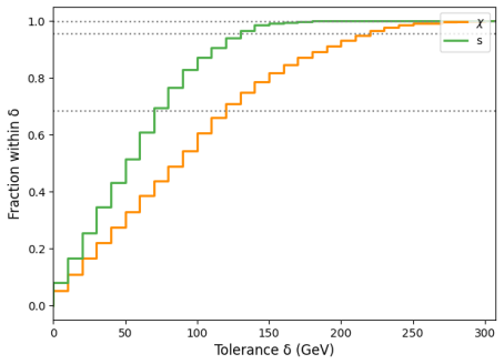
The central claim is that the same CNN architecture can solve three related characterization tasks on distributions reconstructed at detector level. On mono-jet data (transverse momentum, missing transverse energy, pseudorapidity) the classifier separates one-component from two-component dark matter signals with roughly 70% accuracy on the two-component class, and the regressors recover the masses: within about 50–80 GeV at 68% tolerance for single-component scalar/fermion signals and about 100 GeV for two-component signals. On mono-Z data, the same network also uses the angular separation Δφ between the two leptons to distinguish a single scalar from a single fermion, and mass estimates tig
What carries the argument
The engine of the analysis is an n-observable one-dimensional CNN (n-1DCNN). Each reconstructed kinematic variable—pT, missing transverse energy, η, and (for mono-Z) Δφ—is binned into a histogram, and these histograms are fed as separate channels into 1D convolutional layers with dropout and max-pooling, followed by flattening and dense layers so correlations between observables can be re-learned. The design is deliberately extensible to more observables or more final states. Around it, two choices make the learning problem well-posed: the training data are normalized shape-only distributions, and the model parameters are restricted (via a cross-section-ratio condition and coupling rescaling
Load-bearing premise
The results assume a signal-only environment in which both dark matter components are produced with nearly equal cross sections (within 15%) and the couplings are rescaled per mass point; if real data contains Standard Model backgrounds or one component dominates production, the network's classifications and mass estimates are not guaranteed to transfer.
What would settle it
Retrain or re-evaluate the same classifier and regressors on samples that include the usual LHC backgrounds (Z→νν+jets, W→lν+jets) or on samples with a 5:1 cross-section imbalance between the two components (the r=5 case the paper generated but did not report). If the two-component classification accuracy and the stated 68% mass tolerances fall to chance level under either change, the background-free, balanced-training condition is the actual driver of the claim.
If this is right
- If the claim holds, mono-jet data alone is enough to determine that a would-be dark matter signal contains two components and to give a rough mass for each (of order 100 GeV at 68% tolerance).
- Mono-Z adds the spin axis: a one-component signal can be assigned to a spin-1/2 fermion or a spin-0 scalar, and mass precision improves, especially for the scalar.
- Because the CNN consumes histograms, it is a natural fit for detector-level summary statistics and can be extended to more observables (e.g., additional jets or leptons) without architectural redesign.
- The two-stage workflow (classify first, then regress) means the spin and component-count decisions are made once, and the mass estimators never have to hedge across classes.
- The quoted precisions are best-case, signal-only values; a realistic analysis with backgrounds can reasonably expect worse performance, as the paper itself warns.
Where Pith is reading between the lines
- A natural extension would be to inject standard-model backgrounds (Z→νν+jets, W→lν+jets, top-quark pairs) and evaluate how the 70% and 68% numbers degrade; the paper's own caveat implies they will.
- The two-component mono-Z mass bias toward low values suggests kinematic degeneracy or partial dominance of one component; a test is to train on varied cross-section ratios r=2, 3, 5 (the paper generated such points but reports mainly r=1) and see whether the bias tracks r.
- Spin discrimination is only demonstrated for one-component signals; in a mixed two-component sample, the Δφ distribution would contain contributions from both spin channels, and disentangling them is a further problem the present architecture does not address.
- The histogram-based n-1DCNN also suggests a way to use the same data representation for simulation-based inference (likelihood-free posteriors) rather than point estimates, which the paper explicitly leaves for future work.
Editorial analysis
A structured set of objections, weighed in public.
Referee Report
Summary. This paper studies a two-component DM model with a Dirac fermion chi and a real scalar S plus a scalar mediator. The authors generate LO mono-jet and mono-Z events with MadGraph/Pythia/Delphes, normalize histograms of pT, MET, eta (and Delta-phi for mono-Z), and train a multi-channel 1D CNN to (i) classify events as one-component fermion, one-component scalar, or two-component DM; (ii) regress the DM mass(es). All results are presented under a background-free hypothesis and the paper is explicitly framed as a proof-of-concept (Abstract; Sec. 1; Sec. 4; Sec. 5). The main reported findings are: mono-jet classifiers distinguish two-component from one-component signals with roughly 70% recall for the two-component class (Fig. 13); mono-Z classifiers also separate one-component fermion from scalar; mass regression achieves best performance for one-component mono-Z and degrades substantially for two-component signals, with 68% tolerances of order 100 GeV in mono-jet and 75-125 GeV in mono-Z, and 90% tolerances of 150-250 GeV. The authors conclude that a CNN can infer the presence, mass, and spin of DM components.
Significance. Demonstrating that a CNN can extract DM spin in addition to mass from mono-X events would be a valuable addition to the ML-based dark-sector characterization literature, complementing previous one-component studies (Refs. [17,18]). The paper has real strengths: a detector-level simulation chain, a clearly described network architecture, results averaged over 50 independent training/validation splits, and an explicit statement of the background-free proof-of-concept limitation. However, the central novelty--spin extraction from mono-Z data--is not established because the training samples for fermion and scalar DM have disjoint mass ranges (Table 1). The classification and regression numbers also need interpretation with care: the two-component mono-jet class has only ~70% recall and the two-component mass regressions have 90% tolerances of up to 250 GeV. Because the spin claim is load-bearing and currently confounded, the paper cannot be accepted in its present form.
major comments (4)
- [Table 1 / Sec. 3.1.2 / Sec. 4.2] The mono-Z spin-discrimination result is confounded by the training-data mass ranges. Table 1 lists the one-component mono-Z scalar samples with pole masses in [80,230] GeV and the fermion samples in [230,1000] GeV. These ranges are disjoint apart from a single boundary value. A classifier trained to label 'fermion' vs 'scalar' can therefore separate the classes using mass-correlated kinematic variables (lepton pT, MET, eta, Delta-phi) without learning any spin-dependent feature. The footnote to Table 1 notes that mass ranges differ between one- and two-component cases but does not acknowledge that the fermion and scalar one-component ranges are disjoint. Without a mass-matched test, e.g., overlapping mass windows for both spins, the abstract's claim of 'extracting their spin' is not supported.
- [Sec. 4.2 / Fig. 13] The mono-jet classifier shows roughly 70% recall for true two-component events, with ~30% misclassified as one-component (Fig. 13). The text does not report overall accuracy or per-class precision/recall, yet the conclusions describe the classification as 'high accuracy'. Since 'inferring the presence of two DM particles' is a central claim, the paper should report full quantitative classification metrics with uncertainties over the 50 runs and temper the wording accordingly.
- [Sec. 3.1.1 / Eqs. (8),(10) / Sec. 4.1 footnote] All presented results correspond to r=1, i.e., fermion and scalar cross sections within 15% of each other (Eq. (8)). The paper states that r=2,3,5 data sets were also generated (footnote in Sec. 4.1), but no results for those cases are shown. The practical utility for a generic two-component signal depends on robustness when one component dominates; at minimum the authors should explain why the r>1 data are omitted or add a sensitivity study. Relatedly, since all histograms are normalized to unit area (Sec. 3.2.1), absolute rate information that could help separate components in a real analysis is discarded; this should be stated as an explicit limitation of the proof-of-concept.
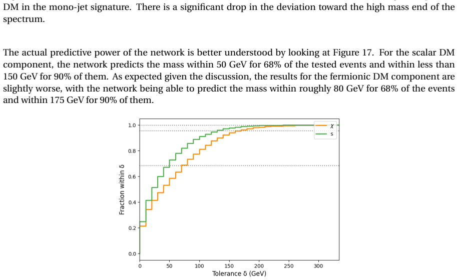
- [Sec. 4.3.2 / Figs. 22,25] Mass extraction in the two-component case is quantitatively modest: mono-jet 68% tolerance is about 100 GeV and 90% tolerance about 250 GeV; mono-Z 68% tolerances are 75 GeV (scalar) and 125 GeV (fermion), with 90% at roughly 225 GeV for the fermion. These numbers should be stated in the abstract or conclusions when claiming that the CNN can 'extract' the DM masses, so that readers can judge the precision. The point estimates are also presented without calibrated uncertainties, which makes the regression claim difficult to interpret.
minor comments (5)
- [Title / Sec. 4.1] Typos and formatting: 'Mono-XSignal' in the title should be 'Mono-X Signal'; the Sec. 4.1 heading 'Then obs-channel 1-Dimensional CNN' should likely read 'The n-obs-channel 1-Dimensional CNN'.
- [Table 1] The caption should explicitly state that the mono-Z one-component fermion and scalar mass ranges are disjoint, since this is crucial for interpreting the spin-classification result.
- [Sec. 3.1.2] After promoting the DM fields to SU(2)_L doublets, referring to Eq. (7) (written for singlet fields) is confusing. The doublet Lagrangian should be written out explicitly or the notation should be clarified.
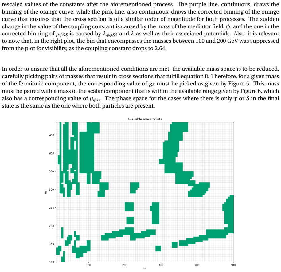
- [Fig. 5 caption] The phrase 'the bin that encompasses the masses between 100 and 200 GeV was suppressed from the plot for visibility' is unclear. Please state what is suppressed, why, and how the reader should interpret the plot.
- [Sec. 4.3.1] The statement that for mono-Z scalar DM 'the network predicts the mass with no deviation for nearly 85% of the tested events' must mean 'within some small tolerance'; the wording should be corrected to avoid implying exact predictions.
Circularity Check
Mono-Z spin classification is confounded with disjoint one-component mass ranges, so the spin-extraction claim reduces to mass-threshold classification by construction.
specific steps
-
other
[Table 1 (Section 3.1.2); Section 4.2]
"Table 1 ... Mono-Z ... 1DM mχ ∈ [230, 1000] GeV; ms ∈ [80,230] GeV ... Notice that, for the mono-Z signature, the mass ranges differ between the one- and two-component DM cases. ... When dealing with mono-Z events, it is expected for the network to be able to distinguish between the spins of the particles in the one-component DM case, given the angular distance between the two leptons in the final state."
The one-component fermion and scalar mono-Z samples are defined on disjoint pole-mass intervals (fermions ≥230 GeV, scalars ≤230 GeV). Thus the spin label is perfectly determined by the mass label in the training data. The CNN's mono-Z spin discrimination accuracy can be reproduced by any mass-correlated kinematic threshold (e.g., on pT or MET); the reported performance does not isolate Δφ or any spin-sensitive observable. Because no mass-matched fermion/scalar control is presented, the 'spin extraction' result is an artifact of the training-data construction rather than evidence of spin sensitivity.
full rationale
The paper is otherwise a self-contained supervised-learning benchmark: events are simulated with MadGraph/Pythia/Delphes, regressors and classifiers are evaluated on held-out test sets drawn from the same mass points, and the cross-section balancing condition (Eq. 8) and coupling rescaling (Eq. 10) are openly stated modeling assumptions, not hidden fits to the target claims. Mass regression and one-vs-two-component classification do not reduce by construction. No load-bearing self-citation chain is used. The single significant circularity is the mono-Z spin claim: Table 1 assigns non-overlapping mass ranges to the fermion and scalar one-component samples, making spin and mass labels identical by construction. The classifier therefore need not use any spin-dependent information, and the abstract's claim of extracting spin is not demonstrated. This is partial circularity, not a fully circular derivation.
Axiom & Free-Parameter Ledger
free parameters (6)
- g_S(m_chi) per mass bin (mono-jet) =
7.4e-6 to 2.94 (Table 1)
- mu_phiSS(m_S) per mass bin (mono-jet) =
4.2e-8 to 1200 (Table 1)
- Cross-section ratio parameter r =
1, 2, 3, 5 (main results r=1)
- Fixed couplings for mono-Z (g_S, mu_phiSS) =
g_S=0.2, mu_phiSS=125 GeV
- NN hyperparameters (learning rate, filters, early stopping patience) =
learning rate 1e-4 to 1e-3; filters/patience vary
- Mixing angle alpha and fixed quartic couplings (lambda, lambda_phi_phiSS) =
alpha small (<4-10% from Refs [41-43]); lambda=0.01/0.057, lambda_phi_phiSS=0.02
axioms (5)
- domain assumption Two-component DM model of Ref. [24] (fermion chi, scalar S, scalar mediator phi, one Z2 symmetry)
- domain assumption Signal-only (background-free) hypothesis for both mono-jet and mono-Z
- ad hoc to paper Normalized histogram shapes (not absolute rates) contain sufficient information
- domain assumption Validity of the Monte Carlo toolchain (SARAH/SPHENO/MadGraph/PYTHIA/Delphes) for LO simulation and detector response
- domain assumption Small mixing angle alpha between Higgs and mediator, satisfying Ref. [41] constraints
invented entities (1)
-
SU(2)_L doublet dark fermion chi and dark scalar S (mono-Z realization)
no independent evidence
Cite this review
Pith. "Pith review of Mono-X Signal Characterization from Two-component Dark Matter Using a Convolutional Neural Network." pith.science (2026). https://pith.science/paper/4TH4KP3J
@misc{pith2026260803975,
  author       = {Pith},
  title        = {Pith review of: Mono-X Signal Characterization from Two-component Dark Matter Using a Convolutional Neural Network},
  year         = {2026},
  howpublished = {\url{https://pith.science/paper/4TH4KP3J}},
  note         = {Machine review of arXiv:2608.03975}
}
read the original abstract
We assess the scope of a Convolutional Neural Network (CNN) in characterizing potential signals of two-component Dark Matter (DM) arising at the Large Hadron Collider (LHC) from mono-jet and mono-Z probes. We show that such a CNN has the ability of not only inferring the presence of two DM particles but also of extracting their mass and spin, the latter being either 0 or 1/2, following detector level analysis. However, such result represents a conceptual proof-of-concept, as we have not entertained a signal-to-background analysis.
Figures








Reference graph
Works this paper leans on
- [1]
-
[2]
V . C. Rubin and W . K. Ford, Jr., Astrophys. J.159(1970), 379-403
work page 1970
-
[3]
E. Corbelli and P . Salucci, Mon. Not. Roy. Astron. Soc.311(2000), 441-447 [arXiv:astro-ph/9909252 [astro- ph]]
Pith/arXiv arXiv 2000
-
[4]
D. Clowe, M. Bradac, A. H. Gonzalez, M. Markevitch, S. W . Randall, C. Jones and D. Zaritsky, Astrophys. J. Lett.648(2006), L109-L113 [arXiv:astro-ph/0608407 [astro-ph]]
Pith/arXiv arXiv 2006
-
[5]
N. Aghanimet al.[Planck], Astron. Astrophys.641(2020), A6 [erratum: Astron. Astrophys.652(2021), C4] [arXiv:1807.06209 [astro-ph.CO]]
Pith/arXiv arXiv 2020
-
[6]
G. Bertone, D. Hooper and J. Silk, Phys. Rept.405(2005), 279-390. [arXiv:hep-ph/0404175 [hep-ph]]
Pith/arXiv arXiv 2005
-
[7]
O. Buchmueller, C. Doglioni and L. T . Wang, Nature Phys.13(2017) no.3, 217-223 [arXiv:1912.12739 [hep- ex]]
Pith/arXiv arXiv 2017
- [8]
- [9]
-
[10]
M. Koch-Janusz and Z. Ringel, Nature Phys.14(2018) no.6, 578-582 [arXiv:1704.06279 [cond-mat.dis-nn]]
Pith/arXiv arXiv 2018
- [11]
-
[12]
A. J. Brennan, M. F . McDonald, J. Gramling and T . D. Jacques, JHEP05(2016), 112 [arXiv:1603.01366 [hep- ph]]
Pith/arXiv arXiv 2016
-
[13]
S. P . Liew, M. Papucci, A. Vichi and K. M. Zurek, JHEP06(2017), 082 [arXiv:1612.00219 [hep-ph]]
work page internal anchor Pith review Pith/arXiv arXiv 2017
-
[14]
E. Bernreuther, J. Horak, T . Plehn and A. Butter, SciPost Phys.5(2018) no.4, 034 [arXiv:1805.11637 [hep- ph]]
work page internal anchor Pith review Pith/arXiv arXiv 2018
-
[15]
K. Cranmer, J. Brehmer and G. Louppe, Proc. Nat. Acad. Sci.117(2020) no.48, 30055-30062 [arXiv:1911.01429 [stat.ML]]
Pith/arXiv arXiv 2020
- [16]
-
[17]
C. K. Khosa, V . Sanz and M. Soughton, SciPost Phys.10(2021) no.6, 151 [arXiv:1910.06058 [hep-ph]]
work page internal anchor Pith review Pith/arXiv arXiv 2021
-
[18]
E. Arganda, A. D. Medina, A. D. Perez and A. Szynkman, SciPost Phys.12(2022) no.2, 063 [arXiv:2105.12018 [hep-ph]]
Pith/arXiv arXiv 2022
- [19]
-
[20]
H. Lv, D. Wang and L. Wu, Phys. Rev. D106, no.5, 055008 (2022) [arXiv:2203.14569 [hep-ph]]
work page internal anchor Pith review Pith/arXiv arXiv 2022
-
[21]
Boosting mono-jet searches with model-agnostic machine learning
T . Finke, M. Krämer, M. Lipp and A. Mück, JHEP08, 015 (2022) [arXiv:2204.11889 [hep-ph]]
work page internal anchor Pith review Pith/arXiv arXiv 2022
-
[22]
F . Gianotti, M. L. Mangano, T . Virdee, S. Abdullin, G. Azuelos, A. Ball, D. Barberis, A. Belyaev, P . Bloch and M. Bosman,et al.Eur. Phys. J. C39, 293-333 (2005) [arXiv:hep-ph/0204087 [hep-ph]]
Pith/arXiv arXiv 2005
-
[23]
S. Bhattacharya, A. Drozd, B. Grzadkowski and J. Wudka, JHEP10(2013), 158 [arXiv:1309.2986 [hep-ph]]
Pith/arXiv arXiv 2013
-
[24]
S. Esch, M. Klasen and C. E. Yaguna, JHEP09(2014), 108 [arXiv:1406.0617 [hep-ph]]
Pith/arXiv arXiv 2014
-
[25]
M. Aoki and T . Toma, JCAP01(2017), 042 [arXiv:1611.06746 [hep-ph]]
Pith/arXiv arXiv 2017
-
[26]
A Minimal Model For Two-Component FIMP Dark Matter: A Basic Search
S. Peyman Zakeri, S. Mohammad Moosavi Nejad, M. Zakeri and S. Yaser Ayazi, Chin. Phys. C42(2018) no.7, 073101 [arXiv:1801.09115 [hep-ph]]
work page internal anchor Pith review Pith/arXiv arXiv 2018
-
[27]
Two-component dark matter and a massless neutrino in a new B-L model
N. Bernal, D. Restrepo, C. Yaguna and Ó. Zapata, Phys. Rev. D99(2019) no.1, 015038 [arXiv:1808.03352 [hep-ph]]
work page internal anchor Pith review Pith/arXiv arXiv 2019
-
[28]
Minimal Two-component Scalar Doublet Dark Matter with Radiative Neutrino Mass
D. Borah, R. Roshan and A. Sil, Phys. Rev. D100(2019) no.5, 055027 [arXiv:1904.04837 [hep-ph]]
work page internal anchor Pith review Pith/arXiv arXiv 2019
-
[29]
A. Aranda, D. Hernández-Otero, J. Hernández-Sanchez, V . Keus, S. Moretti, D. Rojas-Ciofalo and T . Shin- dou, Phys. Rev. D103, no.1, 015023 (2021) [arXiv:1907.12470 [hep-ph]]
Pith/arXiv arXiv 2021
-
[30]
The $Z_5$ model of two-component dark matter
G. Bélanger, A. Pukhov, C. E. Yaguna and Ó. Zapata, JHEP09(2020), 030 [arXiv:2006.14922 [hep-ph]]
work page internal anchor Pith review Pith/arXiv arXiv 2020
-
[31]
Multi-component Dark Matter in a Simplified E$_6$SSM Model
S. Khalil, S. Moretti, D. Rojas-Ciofalo and H. Waltari, Phys. Rev. D102(2020) no.7, 075039 [arXiv:2007.10966 [hep-ph]]
work page internal anchor Pith review Pith/arXiv arXiv 2020
-
[32]
Two Component Doublet-Triplet Scalar Dark Matter stabilising the Electroweak vacuum
N. Chakrabarty, R. Roshan and A. Sil, Phys. Rev. D105(2022) no.11, 115010 [arXiv:2102.06032 [hep-ph]]
work page internal anchor Pith review Pith/arXiv arXiv 2022
-
[33]
C. E. Yaguna and Ó. Zapata, Phys. Rev. D105(2022) no.9, 095026 [arXiv:2112.07020 [hep-ph]]
work page internal anchor Pith review Pith/arXiv arXiv 2022
-
[34]
The $Z_3$ soft breaking in the I(2+1)HDM and its probes at present and future colliders
D. Hernández-Otero, J. Hernández-Sánchez, S. Moretti and T . Shindou, [arXiv:2203.06323 [hep-ph]]
work page internal anchor Pith review Pith/arXiv arXiv
-
[35]
J. Hernandez-Sanchez, V . Keus, S. Moretti, D. Rojas-Ciofalo and D. Sokolowska, [arXiv:2012.11621 [hep- ph]]
Pith/arXiv arXiv 2012
-
[36]
J. Hernandez-Sanchez, V . Keus, S. Moretti and D. Sokolowska, JHEP03, 045 (2023) [arXiv:2202.10514 [hep- ph]]
Pith/arXiv arXiv 2023
-
[37]
A combined approach to the analysis of space and ground experimental data within a simplified E6SSM
S. Khalil, K. Kowalska, S. Moretti, D. Rojas-Ciofalo and H. Waltari, Eur. Phys. J. C82, no.11, 1058 (2022) [arXiv:2107.10780 [hep-ph]]
work page internal anchor Pith review Pith/arXiv arXiv 2022
-
[38]
M. Aoki, M. Duerr, J. Kubo and H. Takano, Phys. Rev. D86(2012), 076015 [arXiv:1207.3318 [hep-ph]]
work page internal anchor Pith review Pith/arXiv arXiv 2012
-
[39]
C. E. Yaguna and Ó. Zapata, JHEP03(2020), 109 [arXiv:1911.05515 [hep-ph]]
work page internal anchor Pith review Pith/arXiv arXiv 2020
-
[40]
G. Bélanger, A. Pukhov, C. E. Yaguna and Ó. Zapata, JHEP03(2023), 100 [arXiv:2212.07488 [hep-ph]]
Pith/arXiv arXiv 2023
-
[41]
Barateet al.[LEP Working Group for Higgs boson searches, ALEPH, DELPHI, L3 and OPAL], Phys
R. Barateet al.[LEP Working Group for Higgs boson searches, ALEPH, DELPHI, L3 and OPAL], Phys. Lett. B565(2003), 61-75 [arXiv:hep-ex/0306033 [hep-ex]]
Pith/arXiv arXiv 2003
-
[42]
G. Aadet al.[ATLAS], Phys. Rev. D101(2020) no.1, 012002 [arXiv:1909.02845 [hep-ex]]
Pith/arXiv arXiv 2020
-
[43]
Tumasyanet al.[CMS], Nature607(2022) no.7917, 60-68 [arXiv:2207.00043 [hep-ex]]
A. Tumasyanet al.[CMS], Nature607(2022) no.7917, 60-68 [arXiv:2207.00043 [hep-ex]]
Pith/arXiv arXiv 2022
-
[44]
Dark Matter Spin Characterisation in Mono-$Z$ Channels
W . Abdallah, A. Hammad, S. Khalil and S. Moretti, Phys. Rev. D100(2019) no.9, 095006 [arXiv:1907.08358 [hep-ph]]
work page internal anchor Pith review Pith/arXiv arXiv 2019
- [45]
-
[46]
F . Staub, Comput. Phys. Commun.184(2013), 1792-1809 [arXiv:1207.0906 [hep-ph]]
Pith/arXiv arXiv 2013
-
[47]
F . Staub, Comput. Phys. Commun.185(2014), 1773-1790 [arXiv:1309.7223 [hep-ph]]
Pith/arXiv arXiv 2014
-
[48]
W . Porod, Comput. Phys. Commun.153(2003), 275-315 [arXiv:hep-ph/0301101 [hep-ph]]
Pith/arXiv arXiv 2003
-
[49]
W . Porod and F . Staub, Comput. Phys. Commun.183(2012), 2458-2469 [arXiv:1104.1573 [hep-ph]]
Pith/arXiv arXiv 2012
-
[50]
J. Alwall, R. Frederix, S. Frixione, V . Hirschi, F . Maltoni, O. Mattelaer, H. S. Shao, T . Stelzer, P . Torrielli and M. Zaro, JHEP07, 079 (2014) [arXiv:1405.0301 [hep-ph]]
Pith/arXiv arXiv 2014
-
[51]
T . Sjostrand, S. Mrenna and P . Z. Skands, Comput. Phys. Commun.178(2008), 852-867 [arXiv:0710.3820 [hep-ph]]
Pith/arXiv arXiv 2008
-
[52]
T . Sjöstrand, S. Ask, J. R. Christiansen, R. Corke, N. Desai, P . Ilten, S. Mrenna, S. Prestel, C. O. Rasmussen and P . Z. Skands, Comput. Phys. Commun.191(2015), 159-177 [arXiv:1410.3012 [hep-ph]]
Pith/arXiv arXiv 2015
-
[53]
de Favereauet al.[DELPHES 3], JHEP02(2014), 057 [arXiv:1307.6346 [hep-ex]]
J. de Favereauet al.[DELPHES 3], JHEP02(2014), 057 [arXiv:1307.6346 [hep-ex]]
Pith/arXiv arXiv 2014
-
[54]
E. Conte, B. Fuks and G. Serret, Comput. Phys. Commun.184, 222-256 (2013) [arXiv:1206.1599 [hep-ph]]
Pith/arXiv arXiv 2013
-
[55]
J. Brehmer, G. Louppe, J. Pavez and K. Cranmer, Proc. Nat. Acad. Sci.117(2020) no.10, 5242-5249 [arXiv:1805.12244 [stat.ML]]
Pith/arXiv arXiv 2020
-
[56]
A. Hallin, J. Isaacson, G. Kasieczka, C. Krause, B. Nachman, T . Quadfasel, M. Schlaffer, D. Shih and M. Som- merhalder, Phys. Rev. D106(2022) no.5, 055006 [arXiv:2109.00546 [hep-ph]]
Pith/arXiv arXiv 2022
-
[57]
B. Nachman and J. Thaler, Phys. Rev. D103(2021) no.11, 116013 [arXiv:2101.07263 [physics.data-an]]
Pith/arXiv arXiv 2021
-
[58]
L. Heinrich, S. Mishra-Sharma, C. Pollard and P . Windischhofer, [arXiv:2306.12584 [stat.ML]]
-
[59]
E. M. Metodiev, B. Nachman and J. Thaler, JHEP10(2017), 174 [arXiv:1708.02949 [hep-ph]]
Pith/arXiv arXiv 2017
-
[60]
B. Nachman and D. Shih, Phys. Rev. D101(2020), 075042 [arXiv:2001.04990 [hep-ph]]
Pith/arXiv arXiv 2020
-
[61]
G. Papamakarios, E. Nalisnick, D. J. Rezende, S. Mohamed and B. Lakshminarayanan, J. Machine Learning Res.22(2021) no.1, 2617-2680 [arXiv:1912.02762 [stat.ML]]
Pith/arXiv arXiv 2021
-
[62]
G. Papamakarios, T . Pavlakou and I. Murray, [arXiv:1705.07057 [stat.ML]]. 22
discussion (0)
Sign in with ORCID, Apple, or X to comment. Anyone can read and Pith papers without signing in.