Improved Physics-informed neural networks loss function regularization with a variance-based term

Hugues Talbot; Irene E. Vignon-Clementel; John M. Hanna

REVIEW 3 major objections 5 minor 36 references

Improved Physics-informed neural networks loss function regularization with a variance-based term

T0 review · 3 major / 5 minor · reviewed 2026-08-11 · deepseek-v4-flash

Challenge this review Re-run · record.json Download PDF Read on arXiv ↗ Review JSON

Pith's one-line read A PINN loss that combines the mean and the standard deviation of pointwise errors produces more uniform error fields and lower maximum errors than minimizing the mean alone.

desk verdict A simple, plausible one-line loss for PINNs, but the evidence is under-powered by test-tuned alpha and single runs; worth refereeing, not yet citable. read the letter →

arxiv 2412.13993 v3 pith:4TLFGQPQ submitted 2024-12-18 math.OC cs.LG

John M. Hanna , Hugues Talbot , Irene E. Vignon-Clementel This is my paper · ORCID

classification math.OCcs.LG MSC 68T0765N35

keywords physics-informedneuralnetworkslossfunctionstandarddeviationvarianceregularizationerrordistributionmaximumcollocationpointspartialdifferentialequations

verification ladder T0 review T1 audit T2 compute T3 formal

The pith

A machine-rendered reading of the paper's core claim, the machinery that carries it, and where it could break.

The reading

Physics-informed neural networks (PINNs) solve partial differential equations by minimizing a loss that averages pointwise errors over collocation and boundary points, but a mean-based loss tolerates large localized errors wherever the solution has steep gradients. This paper claims that adding the standard deviation of those pointwise errors to the loss, so that both the average error and its spread are minimized, forces the network to allocate effort to the worst regions rather than the bulk. On four test problems, from a smooth 1D Poisson equation to a steep Burgers shock and a 2D Navier-Stokes flow, the proposed loss is reported to reduce the maximum absolute error by a factor of about 2 to 30, while adding only a few percent to training time. The paper also reports that the same accuracy can be reached with substantially fewer collocation points, which would matter for expensive high-dimensional problems. The simple form of the loss, one line changed in existing code, is the practical payoff.

What carries the argument

The load-bearing object is the variance-augmented loss of Eq. (12): $L=\alpha\,\mathrm{mean}(e_i)+(1-\alpha)\,\mathrm{std}(e_i)$, with $e_i$ the pointwise squared error of the PDE residual, initial condition, or boundary condition. The mean keeps the overall fit tight; the standard-deviation term smooths the error landscape by making the optimizer reduce the largest deviations, which is what transfers effort to high-gradient regions. $\alpha$, chosen per problem by sweeping from 0 to 1, sets how much weight the spread term receives; best values were 0.8, 0.8, 0.6 and 0.8 across the four tests.

What would settle it

Train the four benchmarks, or a single smooth Poisson case, with the proposed loss and the mean-squared loss across twenty random seeds each, fixing $\alpha=0.8$, and compare maximum pointwise error on the same collocation set; if the variance-based loss does not reach a lower or equal maximum error in a clear majority of seeds, the central claim fails.

Watch

Extended reading notes

Core claim

The central claim is that replacing the usual mean-error loss $L=\frac{1}{N}\sum_i e_i$ with $L=\alpha \frac{1}{N}\sum_i e_i + (1-\alpha)\sqrt{\frac{\sum_i(e_i-\bar e)^2}{N}}$, where $e_i$ is the squared pointwise residual or boundary mismatch and $\alpha$ balances the two terms, yields a more uniform error distribution and a lower maximum error than the mean alone. The standard deviation term penalizes the dispersion of errors, so the optimizer cannot hide a few large residuals inside a small average. In the experiments this shows up as an $L^\infty$ error reduced by roughly 2x on Burgers, 15–30x on the 2D elasticity displacement, and more than 3x on velocity plus an order of magnitude on pressure in the Navier-Stokes case, with best results usually at $\alpha=0.8$. The paper frames the term as regularization, notes that no theoretical justification for the $\alpha$ choice is yet known, and contrasts the method with gradient-enhanced PINNs and Huber loss, finding comparable or better accuracy at a fraction of the computational cost.

Load-bearing premise

The reported gains assume that the per-problem hyperparameter $\alpha$, selected by sweeping its value against a known reference solution, is representative enough that a user can pick it without such a reference; all headline numbers are single runs at the chosen $\alpha$, and no choice rule is given.

Editorial extensions

If this is right

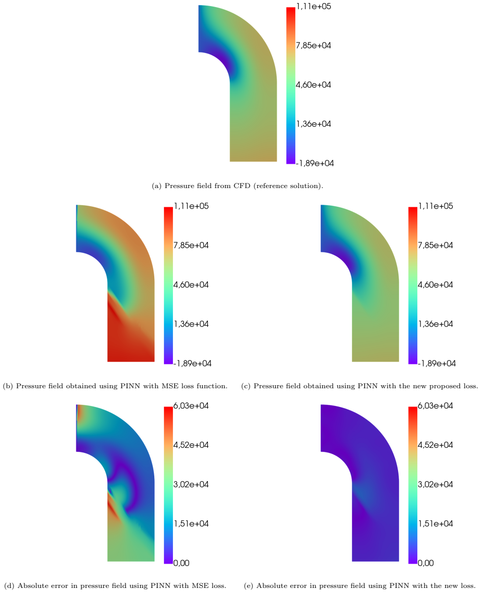
On the four tested problems, the variance-based loss lowers the maximum absolute error compared with mean-squared loss: roughly 2x for Burgers, 15–30x for the elasticity displacements, and an order of magnitude for the Navier-Stokes pressure.
Because the loss is a one-line change in standard frameworks, the improvement comes with negligible added compute: one to two seconds extra on problems that take 8–45 seconds, and about one extra minute on the 15-minute Navier-Stokes run.
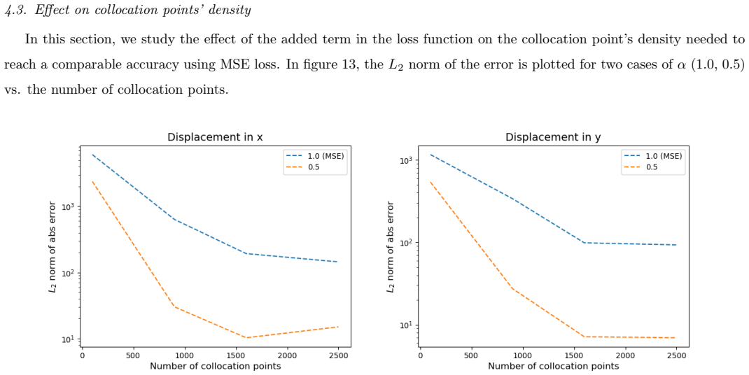
The same target accuracy can be reached with fewer collocation points when the variance term is active, which the paper argues is decisive for high-dimensional or expensive PDE problems.
Against gradient-enhanced PINNs and Huber loss on the elasticity benchmark, the proposed loss matches or approaches the accuracy of gradient-enhanced training while avoiding the multi-fold cost increase and the extra implementation burden.

Reading between the lines

Editorial extensions of the paper, not claims the author makes directly.

Editorial extension: applying the same mean-plus-standard-deviation construction separately to each term of a multi-task PINN loss, such as PDE residual, initial condition, and boundary, would add per-task variance penalties and might outperform the single global $\alpha$ used here.
Editorial extension: because the variance term already pushes optimization toward high-error zones, it should reduce or delay the need for residual-based adaptive sampling; a direct test is to compare adaptive-sampling PINNs with and without the proposed loss at fixed point counts.
Editorial extension: the reported gains grow with problem sharpness—small on smooth Poisson, large on the Burgers front and elasticity corners—so the loss is likely most valuable precisely where mean-squared PINN training is known to struggle.

Share X Bluesky LinkedIn Reddit HN

Signed reviews

No signed human review yet.

Editorial analysis

A structured set of objections, weighed in public.

Desk editor's note, referee report, and a circularity audit.

Desk Editor's Note

read the letter

Short version: the paper's one-line loss change is a legitimate, reproducible idea, and the qualitative results are encouraging. The alpha-tuning and single-run issues are real and should be fixed before this is cited as strong evidence.

The proposal is exactly what it looks like: add the population standard deviation of per-sample residuals to the mean, with weight alpha, as in Eq. (12). That exact combination is not in the cited prior work; VI-PINNs learns a variance output and Markowitz is portfolio selection, so the one-line loss is new in the PINN context. It is trivially implementable, and the reported compute overhead is a few percent. The experiments on four benchmarks show lower max error and cleaner error maps with the variance term. I believe those qualitative observations.

The soft spots are in the evidence, not the idea. Alpha is swept from 0 to 1 on each problem and the best value is read off the test-error curves; all headline numbers are at that chosen alpha. With one initialization shared across the sweep, you are comparing single trajectories, not sampling the optimization landscape. No seeds, no error bars. For Navier-Stokes, the MSE baseline diverges under the fixed Adam setting, so the comparison there is against a failed run, not a healthy baseline. The positive results on Poisson and Burgers are smaller and more believable, but still single runs. The paper admits the choice of alpha is empirical and gives no rule for picking it without a reference solution, which limits the drop-in story.

That said, the paper is not sloppy in its claims: it connects to Markowitz, compares against Huber and gPINNs, and reports computational cost. The writing is clear and the method is simple enough to reproduce. The problem is under-powered validation, not incoherence.

My take: this deserves a serious referee, but it needs revision before acceptance. Ask for multiple seeds, error bars, a pre-specified alpha rule or a sensitivity analysis showing the gain holds across a range of alpha, and a Navier-Stokes baseline that does not diverge. If the max-error reduction survives that, it is a useful contribution. If not, it is a cautionary tale about tuning on the test set.

I would bring it to reading group as a case study in loss-function evaluation. I would not cite it yet.

Referee Report

3 major / 5 minor

Summary. The paper proposes a modified PINN loss function, Eq. (12), that combines the mean of a per-point error with its standard deviation: L = alpha * mean(e_i) + (1-alpha) * std(e_i). The authors argue that penalizing the standard deviation of the residuals, in addition to their mean, reduces localized high-error regions and leads to a more uniform error distribution. The method is tested on four problems: 1D Poisson, unsteady Burgers, 2D linear elasticity, and 2D steady Navier-Stokes. In each case, alpha is swept between 0 and 1 and the best value is selected from error-versus-iteration plots; the authors report reductions in maximum error (about 2x for Burgers, 30x/15x for elasticity, and more than 3x plus an order of magnitude for Navier-Stokes) with negligible additional computational cost. Comparisons with Huber loss and gradient-enhanced PINNs are also presented for the elasticity problem.

Significance. If the reported improvements are robust, the proposed loss is an attractive, one-line modification to PINN training: it is simple to implement, has negligible computational overhead, and could help with problems exhibiting localized errors or sharp gradients. The paper also provides a collocation-density experiment suggesting improved data efficiency and a direct comparison with two existing regularization strategies. The main weakness is that the central claim is empirical and the supporting evidence is currently fragile: the reported gains are measured at per-problem alpha values selected from test-error curves, with a single initialization per configuration and no error bars. The Navier-Stokes comparison is further weakened by the divergence of the MSE baseline. The idea is plausible and potentially useful, but the strength of the claims in the abstract and conclusion is not yet matched by the experimental support.

major comments (3)

[Section 3 (alpha sweep and figures 1, 2, 5, 9)] The headline reductions in maximum error are maxima over alpha: for each problem the best alpha value (0.8, 0.8, 0.6, 0.8) is selected from L2-error-versus-iteration curves computed against the analytical or reference solution, and all subsequent comparisons use this selected value. Because the same Xavier initialization is reused for every alpha, the sweep selects the best of several single trajectories rather than comparing expected performance. No rule is given for choosing alpha without a reference solution, so Eq. (12) contains a free hyperparameter that is fitted to the test error. Multi-seed runs at a fixed alpha, error bars, and a validation-based alpha-selection protocol are needed before the abstract's claim that the loss 'ensures a more uniform error distribution' can be considered supported.
[Section 3.4 (Navier-Stokes example, figure 9)] The MSE baseline (alpha=1) diverges from the reference solution under the fixed Adam setup, and the subsequent pressure and velocity comparisons are made against this failed baseline. The reported order-of-magnitude pressure improvement and the inability of MSE to capture the outlet velocity profile may therefore reflect an unstable or under-converged baseline rather than a genuine benefit of the variance term. The comparison should be repeated with a standard PINN baseline that is known to converge, for example by using more iterations, a learning-rate schedule, or a more powerful optimizer, so that the variance-based loss is measured against a successful standard PINN.
[Section 4.3 (collocation-point density experiment, figure 13)] The efficiency claim that the proposed loss achieves a given accuracy with substantially fewer collocation points rests on only two alpha values and, as far as reported, a single training run per configuration. No repeated-seed statistics or error bars are shown, and the caption repeats 'On the left' for both panels. This is not sufficient support for the conclusion in Section 4.4 that the modified loss reduces reliance on dense spatial sampling; multiple seeds and a clearer comparison of error at matched collocation counts are required.

minor comments (5)

[Throughout] There are several typos and grammatical errors, including 'the our new loss' in Section 3.1, 'Burger's' for 'Burgers'' in several places, and 'krieging' for 'kriging' in the Introduction. A proofreading pass is needed.
[Section 4.2] The comparison with gradient-enhanced PINNs and Huber loss is qualitative: no hyperparameters for gPINNs are given, and the claimed 'marginal improvement' is not quantified. Reporting the final L2 errors for each method would make the comparison more informative.
[Section 3.3] The text states that the new loss is 'always significantly better' than MSE based on Figure 5, but no statistical significance tests are reported and only one run per alpha is shown. The word 'significantly' should either be removed or backed by multi-seed statistics.
[Eq. (12)] The standard deviation is defined with a denominator of N rather than N-1. This is a legitimate choice for a loss term, but it should be stated explicitly since it affects the gradient scale.
[Data and code availability] No statement on code or data availability is included. Given the empirical nature of the claims, releasing the training code and seeds would substantially help reproducibility.

Circularity Check

0 steps flagged · score 0.0 of 10

No significant circularity: the proposed variance-loss is defined independently, and the reported error reductions are empirical comparisons against external analytical and CFD references.

full rationale

The central proposal, Eq. (12), defines L = alpha * mean(e_i) + (1-alpha) * std(e_i). This is an independently stated objective; the paper does not derive the loss from the results it claims to predict. Minimizing standard deviation directly targets error uniformity, but that is a design property of the loss, not a circular proof of the empirical claim of reduced maximum error. The empirical claims are tested against external references: analytical solutions for the 1D Poisson and Burgers problems, an analytical solution for the 2D elasticity problem, and a Fenics CFD reference for the Navier-Stokes problem. These benchmarks are independent of the proposed loss and of the fitted alpha values, so the reported improvements are falsifiable rather than equivalent to the input by construction. The alpha sweep is a genuine methodological limitation: Section 3 states 'we vary alpha from 0 to 1 ... and we have the same initialization ... each time alpha is changed', and best alpha values are selected from the reported error curves. This can inflate the apparent gains and means the reported factors are maxima over the tested alpha grid, but it does not make the central claim circular because the variance term could fail at all alpha values and the external references do not depend on alpha. Self-citations in the reference list (e.g., [16], [18], [22]) are applications of PINNs and are not load-bearing for the loss-function derivation. The conclusion's admission that 'a theoretical justification remains an open question' for alpha is an honest limitation, not a circular step. No equation reduces to its inputs by construction, and no prediction is renamed as a fit.

Assumptions & free parameters 1 free parameters · 3 assumptions · 0 invented entities

The central claim rests on one fitted hyperparameter (alpha), the unproven mechanism that mean+std minimization controls peak errors, and the assumption that a fixed Adam optimizer is a fair comparison. No new physical entities are introduced.

free parameters (1)

alpha = 0.8, 0.8, 0.6, 0.8 per problem
Hyperparameter controlling the relative weight of the mean and standard deviation terms in Eq. (12). Swept from 0 to 1 in increments and selected per problem by minimizing test error; the paper gives no automatic selection rule.

assumptions (3)

standard math The standard PINN residual-minimization framework is valid: the PDE residual loss over collocation points drives the network toward the solution.
Invoked in Section 2.1; relies on Raissi et al. [7] and universal approximation.
ad hoc to paper Penalizing the standard deviation of residuals in addition to their mean reduces the maximum error and makes errors more uniform.
This is the unproven mechanism behind the proposal; Section 4.4 states the theoretical justification remains an open question.
domain assumption The Adam optimizer with fixed learning rate 0.001 is an adequate and fair optimizer for both the baseline and the proposed loss.
The Navier-Stokes baseline diverges under this setting (Section 3.4), so the comparison may depend on this assumption.

how reviews work

0 comments

Cite this review

Pith. "Pith review of Improved Physics-informed neural networks loss function regularization with a variance-based term." pith.science (2026). https://pith.science/paper/4TLFGQPQ

@misc{pith2026241213993,
  author       = {Pith},
  title        = {Pith review of: Improved Physics-informed neural networks loss function regularization with a variance-based term},
  year         = {2026},
  howpublished = {\url{https://pith.science/paper/4TLFGQPQ}},
  note         = {Machine review of arXiv:2412.13993}
}

read the original abstract

In machine learning and statistical modeling, the mean square or absolute error is commonly used as an error metric, also called a "loss function." While effective in reducing the average error, this approach may fail to address localized outliers, leading to significant inaccuracies in regions with sharp gradients or discontinuities. This issue is particularly evident in physics-informed neural networks (PINNs), where such localized errors are expected and affect the overall solution. To overcome this limitation, we propose a novel loss function that combines the mean and the standard deviation of the chosen error metric. By minimizing this combined loss function, the method ensures a more uniform error distribution and reduces the impact of localized high-error regions. The proposed loss function is easy to implement and tested on problems of varying complexity: the 1D Poisson equation, the unsteady Burgers' equation, 2D linear elastic solid mechanics, and 2D steady Navier-Stokes equations. Results demonstrate improved solution quality and lower maximum error compared to the standard mean-based loss, with minimal impact on computational time.

Figures

Figures reproduced from arXiv: 2412.13993 by the authors.

**Figure 1.** On the left, the L2 norm of the absolute error vs. the number of iterations for different values of α for the 1D Poisson example. On the right, a plot of the analytical solution along with the PINN solution for the best α (0.8). As shown in figure 1, the best solution is obtained with an α value of 0.8: adding the variance of the error does improve the accuracy of the prediction. However, the gain in accuracy is not… view at source ↗

**Figure 2.** L2 norm of the absolute solution error vs iterations for different values of α for the Burgers’ problem. The effect of the added extra term is this time quite pronounced. It can be seen that solutions with α = 0.4, 0.6, 0.8 perform better than the classical loss value (α = 1), where the best solution is obtained with α = 0.8. The analytical and PINN solutions in time and space, along with the corresponding absolute … view at source ↗

**Figure 3.** Burger’s equation solutions (time in the x-axis; space in the y-axis), (a) analytical, using both (b) classical mean loss ( [PITH_FULL_IMAGE:figures/full_fig_p009_3.png] view at source ↗

Figures from the paper (10 more)

**Figure 4.** Figure 4: Solid mechanics problem setup and boundary conditions [10]. [PITH_FULL_IMAGE:figures/full_fig_p010_4.png]

**Figure 5.** Figure 5: The L2 norm of the absolute error of x-displacement (left) and y-displacement (right), vs. the number of iterations for different values of α for the 2D linear elasticity example. As can be noticed from figure 5, using the new loss function is always significantly bett…

**Figure 6.** Figure 6: ux analytical solution along with solutions from PINN using MSE loss (α = 1) and the new variance-based loss (α = 0.6), along with the absolute errors. 12 [PITH_FULL_IMAGE:figures/full_fig_p012_6.png]

**Figure 7.** Figure 7: uy analytical solution along with solutions from PINN using MSE loss (α = 1) and the new variance-based loss (α = 0.6), along with the absolute errors. From figures 6 and 7, it is clear that using the newly proposed loss function provides better solutions than using a …

**Figure 8.** Figure 8: Fluid mechanics problem geometry and boundary conditions. [PITH_FULL_IMAGE:figures/full_fig_p014_8.png]

**Figure 9.** Figure 9: On the left, the L2 norm of the absolute error of the pressure vs. the number of iterations for different values of α for the 2D Navier-Stokes example. On the right, the L2 norm of the absolute error of velocity magnitude vs. the number of iterations for different valu…

**Figure 10.** Figure 10: Velocity magnitude using Fenics as a reference solution along with solutions from PINN using MSE loss ( [PITH_FULL_IMAGE:figures/full_fig_p016_10.png]

**Figure 11.** Figure 11: Pressure fields using CFD (reference solution), PINN with MSE loss ( [PITH_FULL_IMAGE:figures/full_fig_p017_11.png]

**Figure 12.** Figure 12: On the left, the L2 norm of the absolute error of x-displacement vs. the number of iterations for different values of α for the 2D linear elasticity example along with gPINNs and Huber loss solutions. On the right, the L2 norm of the absolute error of x-displacement v…

**Figure 13.** Figure 13: On the left, the L2 norm of the absolute error of x-displacement vs. the number of collocation points for α values 1.0 and 0.5, for the 2D linear elasticity example. On the left, the L2 norm of the absolute error of y-displacement vs. the number of collocation points …

Discussion (0). Continue with ORCID to comment.

Reference graph

Works this paper leans on

36 extracted references · 19 canonical work pages

[1]

Z. Wu, S. Pan, F. Chen, G. Long, C. Zhang, S. Y. Philip, A comprehensive survey on graph neural networks, IEEE transactions on neural networks and learning systems 32 (1) (2020) 4–24

work page 2020
[2]

Zhang, L

X.-M. Zhang, L. Liang, L. Liu, M.-J. Tang, Graph neural networks and their current applications in bioinformatics, Frontiers in genetics 12 (2021) 690049

work page 2021
[3]

W. Fan, Y. Ma, Q. Li, Y. He, E. Zhao, J. Tang, D. Yin, Graph neural networks for social recommendation, in: The world wide web conference, 2019, pp. 417–426

2019
[4]

Vaswani, Attention is all you need, Advances in Neural Information Processing Systems (2017)

A. Vaswani, Attention is all you need, Advances in Neural Information Processing Systems (2017)

2017
[5]

T. Wolf, L. Debut, V. Sanh, J. Chaumond, C. Delangue, A. Moi, P. Cistac, T. Rault, R. Louf, M. Funtowicz, et al., Transformers: State-of-the-art natural language processing, in: Proceedings of the 2020 conference on empirical methods in natural language processing: system demonstrations, 2020, pp. 38–45

2020
[6]

K. Han, Y. Wang, H. Chen, X. Chen, J. Guo, Z. Liu, Y. Tang, A. Xiao, C. Xu, Y. Xu, et al., A survey on vision transformer, IEEE transactions on pattern analysis and machine intelligence 45 (1) (2022) 87–110

2022
[7]

Raissi, P

M. Raissi, P. Perdikaris, G. E. Karniadakis, Physics-informed neural networks: A deep learning framework for solving forward and inverse problems involving nonlinear partial differential equations, Journal of Computational Physics 378 (2019) 686–707

2019
[8]

Hornik, M

K. Hornik, M. Stinchcombe, H. White, Multilayer feedforward networks are universal approximators, Neural networks 2 (5) (1989) 359–366

1989

Show all 36 references

[9]

A. G. Baydin, B. A. Pearlmutter, A. A. Radul, J. M. Siskind, Automatic differentiation in machine learning: a survey, Journal of machine learning research 18 (2018)

2018
[10]

Haghighat, M

E. Haghighat, M. Raissi, A. Moure, H. Gomez, R. Juanes, A physics-informed deep learning framework for inversion and surrogate modeling in solid mechanics, Computer Methods in Applied Mechanics and Engineering 379 (2021) 113741

2021
[11]

H. Moon, D. Park, H. Cho, H.-K. Noh, J. H. Lim, S. Ryu, Physics-informed neural network-based discovery of hy- perelastic constitutive models from extremely scarce data, Computer Methods in Applied Mechanics and Engineering 20 446 (2025) 118258.doi:https://doi.org/10.1016/j.cm...

2025
[12]

Z. Mao, A. D. Jagtap, G. E. Karniadakis, Physics-informed neural networks for high-speed flows, Computer Methods in Applied Mechanics and Engineering 360 (2020) 112789

2020
[13]

S. Cai, Z. Mao, Z. Wang, M. Yin, G. E. Karniadakis, Physics-informed neural networks (pinns) for fluid mechanics: A review, Acta Mechanica Sinica (2022) 1–12

2022
[14]

Raissi, A

M. Raissi, A. Yazdani, G. E. Karniadakis, Hidden fluid mechanics: Learning velocity and pressure fields from flow visualizations, Science 367 (6481) (2020) 1026–1030

2020
[15]

Orera, J

J. Orera, J. Ramírez, P. García-Navarro, J. Murillo, Roepinns: An integration of advanced cfd solvers with physics- informed neural networks and application in arterial flow modeling, Computer Methods in Applied Mechanics and Engineering 440 (2025) 117933.doi:https://doi.org/1...

2025
[16]

J. M. Hanna, J. V. Aguado, S. Comas-Cardona, R. Askri, D. Borzacchiello, Residual-based adaptivity for two-phase flow simulation in porous media using physics-informed neural networks, Computer Methods in Applied Mechanics and Engineering 396 (2022) 115100

2022
[17]

M. M. Almajid, M. O. Abu-Al-Saud, Prediction of porous media fluid flow using physics informed neural networks, Journal of Petroleum Science and Engineering 208 (2022) 109205

2022
[18]

J. M. Hanna, J. V. Aguado, S. Comas-Cardona, R. Askri, D. Borzacchiello, Sensitivity analysis using physics-informed neural networks, Engineering Applications of Artificial Intelligence 135 (2024) 108764

2024
[19]

J. Yin, Z. Wen, S. Li, Y. Zhang, H. Wang, Dynamically configured physics-informed neural network in topology optimization applications, Computer Methods in Applied Mechanics and Engineering 426 (2024) 117004.doi:https: //doi.org/10.1016/j.cma.2024.117004. URLhttps://www.scienc...

2024
[20]

Jeong, J

H. Jeong, J. Bai, C. Batuwatta-Gamage, Z. J. Wegert, C. N. Mallon, V. J. Challis, Y. Gui, Y. Gu, Fourier fea- ture embedded physics-informed neural network-based topology optimization (ff-pinnto) framework for geometrically nonlinear structures, Computer Methods in Applied Mec...

2025
[21]

S. A. Niaki, E. Haghighat, T. Campbell, A. Poursartip, R. Vaziri, Physics-informed neural network for modelling the thermochemical curing process of composite-tool systems during manufacture, Computer Methods in Applied Mechanics and Engineering 384 (2021) 113959

2021
[22]

J. M. Hanna, J. V. Aguado, S. Comas-Cardona, Y. Le Guennec, D. Borzacchiello, A self-supervised learning framework based on physics-informed and convolutional neural networks to identify local anisotropic permeability tensor from textiles 2d images for filling pattern predicti...

2024
[23]

Manav, R

M. Manav, R. Molinaro, S. Mishra, L. De Lorenzis, Phase-field modeling of fracture with physics-informed deep learning, Computer Methods in Applied Mechanics and Engineering 429 (2024) 117104

2024
[24]

Goswami, C

S. Goswami, C. Anitescu, S. Chakraborty, T. Rabczuk, Transfer learning enhanced physics informed neural network for phase-field modeling of fracture, Theoretical and Applied Fracture Mechanics 106 (2020) 102447

2020
[25]

Markowitz, Portfolio selection/h

H. Markowitz, Portfolio selection/h. markovitz, The Journal of Finance 7 (1) (1952) 77–91

1952
[26]

D. Nix, A. Weigend, Estimating the mean and variance of the target probability distribution, in: Proceedings of 1994 IEEE International Conference on Neural Networks (ICNN’94), Vol. 1, 1994, pp. 55–60 vol.1.doi:10.1109/ICNN. 1994.374138

1994
[27]

Seeger, Gaussian processes for machine learning, International journal of neural systems 14 (02) (2004) 69–106

M. Seeger, Gaussian processes for machine learning, International journal of neural systems 14 (02) (2004) 69–106

2004
[28]

Matheron, Principles of geostatistics, Economic geology 58 (8) (1963) 1246–1266

G. Matheron, Principles of geostatistics, Economic geology 58 (8) (1963) 1246–1266

1963
[29]

J. Lee, Y. Bahri, R. Novak, S. S. Schoenholz, J. Pennington, J. Sohl-Dickstein, Deep neural networks as gaussian processes, arXiv preprint arXiv:1711.00165 (2017)

2017 arXiv
[30]

P. J. Huber, Robust estimation of a location parameter, in: Breakthroughs in statistics: Methodology and distribution, Springer, 1992, pp. 492–518

1992
[31]

Hastie, The elements of statistical learning: data mining, inference, and prediction, Vol

T. Hastie, The elements of statistical learning: data mining, inference, and prediction, Vol. 2, Springer
[32]

J. Yu, L. Lu, X. Meng, G. E. Karniadakis, Gradient-enhanced physics-informed neural networks for forward and inverse pde problems, Computer Methods in Applied Mechanics and Engineering 393 (2022) 114823

2022
[33]

B. Shan, Y. Li, S.-J. Huang, Vi-pinns: Variance-involved physics-informed neural networks for fast and accurate prediction of partial differential equations, Neurocomputing (2025) 129360

2025
[34]

D. P. Kingma, J. Ba, Adam: A method for stochastic optimization, arXiv preprint arXiv:1412.6980 (2014)

2014 arXiv
[35]

C. G. Broyden, The convergence of a class of double-rank minimization algorithms 1. general considerations, IMA Journal of Applied Mathematics 6 (1) (1970) 76–90

1970
[36]

Basdevant, M

C. Basdevant, M. Deville, P. Haldenwang, J. Lacroix, J. Ouazzani, R. Peyret, P. Orlandi, A. Patera, Spectral and finite difference solutions of the burgers equation, Computers & fluids 14 (1) (1986) 23–41. 22

1986

Pith tools

Reviewed August 11, 2026 · model on record in the stance chip above.

[1] [1]

Z. Wu, S. Pan, F. Chen, G. Long, C. Zhang, S. Y. Philip, A comprehensive survey on graph neural networks, IEEE transactions on neural networks and learning systems 32 (1) (2020) 4–24

work page 2020

[2] [2]

Zhang, L

X.-M. Zhang, L. Liang, L. Liu, M.-J. Tang, Graph neural networks and their current applications in bioinformatics, Frontiers in genetics 12 (2021) 690049

work page 2021

[3] [3]

W. Fan, Y. Ma, Q. Li, Y. He, E. Zhao, J. Tang, D. Yin, Graph neural networks for social recommendation, in: The world wide web conference, 2019, pp. 417–426

2019

[4] [4]

Vaswani, Attention is all you need, Advances in Neural Information Processing Systems (2017)

A. Vaswani, Attention is all you need, Advances in Neural Information Processing Systems (2017)

2017

[5] [5]

T. Wolf, L. Debut, V. Sanh, J. Chaumond, C. Delangue, A. Moi, P. Cistac, T. Rault, R. Louf, M. Funtowicz, et al., Transformers: State-of-the-art natural language processing, in: Proceedings of the 2020 conference on empirical methods in natural language processing: system demonstrations, 2020, pp. 38–45

2020

[6] [6]

K. Han, Y. Wang, H. Chen, X. Chen, J. Guo, Z. Liu, Y. Tang, A. Xiao, C. Xu, Y. Xu, et al., A survey on vision transformer, IEEE transactions on pattern analysis and machine intelligence 45 (1) (2022) 87–110

2022

[7] [7]

Raissi, P

M. Raissi, P. Perdikaris, G. E. Karniadakis, Physics-informed neural networks: A deep learning framework for solving forward and inverse problems involving nonlinear partial differential equations, Journal of Computational Physics 378 (2019) 686–707

2019

[8] [8]

Hornik, M

K. Hornik, M. Stinchcombe, H. White, Multilayer feedforward networks are universal approximators, Neural networks 2 (5) (1989) 359–366

1989