REVIEW 3 major objections 3 minor 89 references
Detecting Atmospheric CO2 Trends as Population-Level Signatures for Long-Term Stable Water Oceans and Biotic Activity on Temperate Terrestrial Exoplanets
T0 review · 3 major / 3 minor · reviewed 2026-08-07 · deepseek-v4-flash
Pith's one-line read The paper argues that a future space-based mid-infrared interferometer could detect the carbonate-silicate CO2 trend in a population of as few as 30 temperate rocky exoplanets, even at S/N = 10 and R = 50.
desk verdict Solid mission-concept simulation for LIFE CO2 trend detection, but the headline detectability claim needs a flat-null control before it is clean. read the letter →
The pith
A machine-rendered reading of the paper's core claim, the machinery that carries it, and where it could break.
The reading
What carries the argument
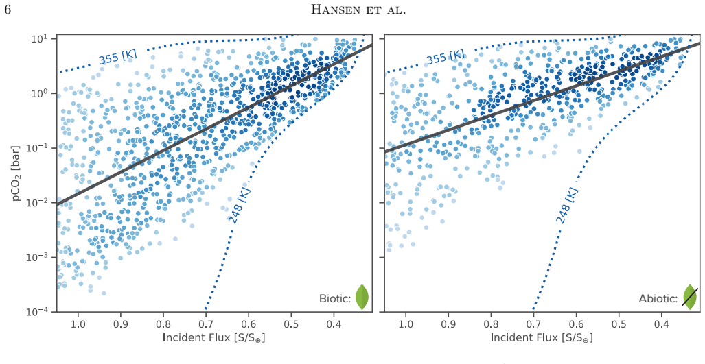
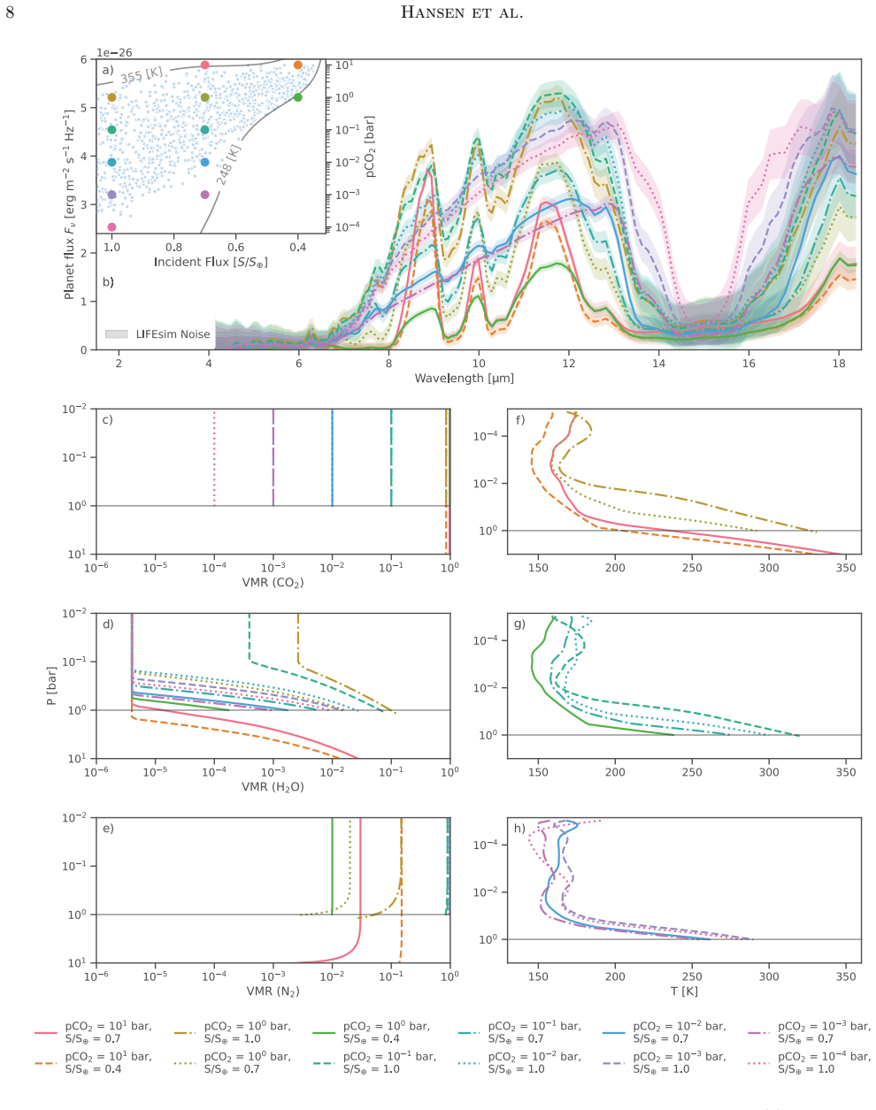
The argument runs through a chain of coupled models and a hierarchical importance-sampling retrieval. Synthetic survey populations are drawn from the Lehmer et al. (2020) coupled geochemistry-climate predictions of the 2D $p\mathrm{CO}_2$-$S$ distribution, with the biotic scenario reproduced from that work and an abiotic scenario obtained by restricting the biological weathering fraction to $[0.1, 0.25]$. A grid of 12 self-consistent climates spanning $p\mathrm{CO}_2 = 10^{-4}$ to $10$ bar and $S/S_\oplus = 0.4$ to $1.0$ is used to generate thermal emission spectra with the ATMOS and petitRADTRANS models, noise-realistic LIFE observations with the LIFEsim simulator, and CO2 posteriors with a Bayesian retrieval. The retrieved posteriors are compressed into maps of Gaussian width $\sigma$ and offset $\Delta$ in the $p\mathrm{CO}_2$-$S$ plane, which assign an observational uncertainty to every synthetic planet. The population trend is then inferred with the hierarchical Bayesian atmospheric retrieval (HBAR) formalism, which reweights each planet's CO2 posterior samples under a semi-logarithmic trend model $\log_{10}(p\mathrm{CO}_2) = \alpha + \beta\,S/S_\oplus$ with scatter $\sigma_N$; comparing the evidence against a flat model yields the Bayes factor used to declare detection.
What would settle it
Run the same pipeline on synthetic populations drawn from a null model with no CO2-flux correlation (uniform pCO2 across the habitable zone, as the paper describes from Lehmer et al. 2020); if the hierarchical retrieval still returns decisive Bayes factors for a linear trend, the detection claim would be an artifact of the retrieval or prior rather than of a real population trend.
Extended reading notes
Core claim
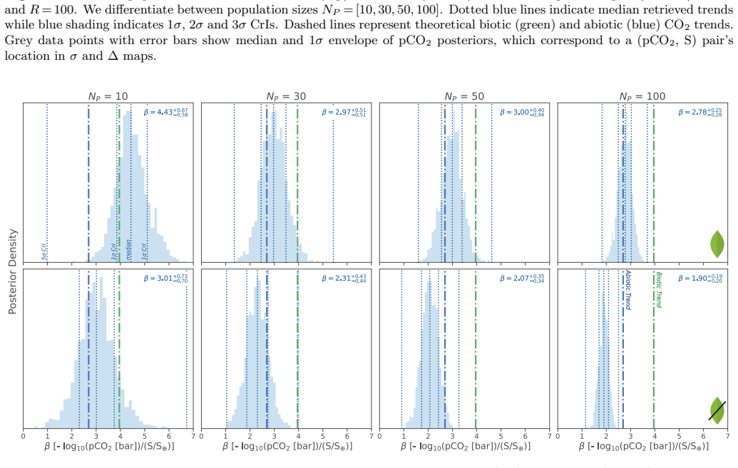
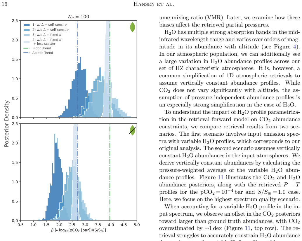
The central claim is that CO2 trends predicted by the carbonate-silicate cycle are observable as population-level signatures with a LIFE-like mid-infrared nulling interferometer. For populations of $N_P \ge 30$ Exo-Earth Candidates and spectrum qualities as low as $S/N = 10$ and $R = 50$, a linear semi-logarithmic trend in $\log_{10}(p\mathrm{CO}_2)$ versus $S/S_\oplus$ is decisively preferred over a flat trend by Bayes factors $\log_{10}(K) > 2$ in both the biotic scenario (biological weathering fraction $f_\mathrm{bio} = 0.1$ to $1.0$) and the abiotic scenario ($f_\mathrm{bio} = 0.1$ to $0.25$). Detecting the trend does not require high spectral resolution or signal-to-noise; population size is the dominant driver. Distinguishing the biotically enhanced from the abiotic trend is harder: systematic offsets in retrieved CO2 partial pressures, traced mainly to the assumption of vertically constant H2O profiles, bias slope estimates toward flatter values, and accurate differentiation would require $N_P \ge 100$ once those biases are corrected.
Load-bearing premise
The whole detectability test assumes the Lehmer et al. (2020) carbonate-silicate model's predicted range of CO2 partial pressures across the habitable zone, and the chosen biotic and abiotic parameter ranges, actually bracket real temperate exoplanet populations; if the real spread is wider, flatter, or shaped differently, the injection-recovery test overstates how easily the trend would be seen.
Editorial extensions
If this is right
- With as few as 30 moderately characterized Exo-Earth Candidates, a LIFE-class mission could decide whether the carbonate-silicate thermostat is operating across a planetary population.
- Detection of the CO2 trend does not hinge on the highest spectral resolutions or signal-to-noise; population size dominates confidence, relaxing mission requirements for this observable.
- If retrieval biases are corrected, populations of about 100 temperate rocky planets could separate trends shaped by global-scale biotic weathering enhancement from abiotic weathering.
- The identified bias from vertically constant H2O profiles affects abundance and pressure constraints across HZ atmospheres, so retrieval frameworks used for population studies must be tested against diverse, non-constant atmospheric profiles.
- Characterizing planets at the hot edge of the habitable zone is intrinsically limited by optically thick, water-rich lower atmospheres, narrowing the accessible population for surface-linked trend studies.
Reading between the lines
- A direct extension suggested by the paper's own logic is to apply the same injection-recovery test to a uniform pCO2-S population (the Lehmer null case), to verify that the Bayes factor does not prefer a linear trend when no trend is injected.
- The trend-slope difference between biotic and abiotic scenarios implies that the slope itself, not just its presence, could serve as a population-level biosignature; correcting the H2O-profile treatment is a concrete path toward using the slope quantitatively.
- The same population-level HBAR machinery could be applied to other spatially or chemically correlated atmospheric signatures, such as CH4-O2 disequilibrium or O3, provided their geochemical null distributions are known.
- Because the paper draws one population per scenario, the reported detection thresholds in the low-$N_P$ regime carry sampling variance; repeating with many population draws would quantify how often a 30-planet survey succeeds.
Editorial analysis
A structured set of objections, weighed in public.
Referee Report
Summary. The paper presents an injection-recovery study of population-level atmospheric CO2 trends as a function of incident stellar flux, using simulated LIFE thermal-emission observations of temperate terrestrial exoplanets. The authors generate synthetic survey populations from LIFE yield simulations, assign pCO2 values from Lehmer et al. (2020) carbonate-silicate cycle predictions for biotic and abiotic scenarios, and compute pCO2 posteriors from 12 atmospheric model scenarios via retrievals. They interpolate these into sigma/delta posterior maps, then use hierarchical Bayesian retrieval following Lustig-Yaeger et al. (2022) to infer a semi-logarithmic trend and compare linear versus flat trend models via Bayes factors. The headline results are that the linear model is decisively preferred for all population sizes and spectral qualities in the biotic case, and for N_P>=30 in the abiotic case, with the claim of 'robust detection'; differentiation of biotic from abiotic trends requires bias correction and N_P>=100. The paper identifies retrieval biases, especially the constant-H2O-profile assumption, as the main source of trend inaccuracy.
Significance. If the detection claim survives the missing null control, the result is significant for the design and science case of LIFE and comparable mid-infrared interferometers: it would show that Cb-Si driven CO2 trends are accessible with about 30 planets even at S/N=10 and R=50, making population-level habitability characterization a realistic goal. The paper is methodologically transparent and reproducible: it uses established public tools (LIFEsim, petitRADTRANS, pyMultiNest, HBAR), provides source data on Zenodo, and clearly separates detection from differentiation while explicitly listing limitations in Section 4.3. Credit is also due for honest discussion of the single-draw caveat, the 12-point grid, the idealized bias correction, and the model-dependence of the biotic/abiotic distinction. However, because the linear-versus-flat comparison has not been tested against a retrieval-bias-only null population, the central quantitative claim is not yet established; the paper's own discussion of S-dependent pCO2 offsets in Section 4.2.1 and Figures 6 and 15 makes such a control necessary.
major comments (3)
- [4.1.1, Eq. (9), Figures 6 and 15] The headline detection claim is not controlled against a retrieval-bias null. The sigma and delta maps in Figures 6 and 15 show that pCO2 posterior offsets are strongly structured in S/S_sun: for pCO2 < 1 bar the offsets grow with incident flux (up to roughly 1 dex at S/S_sun = 1.0), while for pCO2 >= 1 bar they are negative. A true population that is flat in log pCO2 would, after passing through these delta maps and the HBAR likelihood in Eq. (4), produce retrieved posterior medians that trend with S. The linear-over-flat Bayes factor from Eq. (9) could therefore become decisive even when no Cb-Si trend is present. The manuscript only runs the linear-versus-flat comparison on trend-injected populations; a flat-null population has not been pushed through the same sigma/delta maps and HBAR pipeline. Please add this control and report the resulting Bayes factors; if a bias-only population also yields decisive evidence, the N_P>=30 detection claim must be substantially revised or restricted to bias-corrected retrievals.
- [4.1.1, Figure 9] The robust-detection claim for N_P>=30 is supported by a single population draw per (N_P, S/N, R) cell. The text acknowledges that a different draw in the low-N_P regime could change trend detectability, but the abstract and Section 5 state the N_P>=30 result without this caveat. Please report the distribution of log10(K) over many population realizations, at least for the lowest spectrum quality (S/N=10, R=50) and N_P=30, and give the fraction of draws that reach decisive evidence. This is necessary to support the word 'robust' in the central claim.
- [3.2, 4.3] The trend inference relies on sigma and delta maps interpolated from only 12 atmospheric retrievals, with linear interpolation between grid points and nearest-neighbor extrapolation outside them. The injected Lehmer populations place most planets between the three S/S_sun columns and the six pCO2 rows used in the grid, so the interpolated maps are doing substantial work in assigning every planet's posterior. The paper acknowledges in Section 4.3 that the accuracy of this interpolation remains uncertain, but the detection claim depends on it. Please validate the interpolation by running direct retrievals on a sample of off-grid (pCO2, S) pairs, or by comparing interpolated posteriors with a denser grid, and quantify how any interpolation error propagates into the Bayes factors.
minor comments (3)
- [Eq. (9)] The printed expression log10(K) = ln(ZA)-ln(ZB)/ln(10) is missing parentheses; the intended formula is log10(K) = (ln ZA - ln ZB)/ln(10). Please correct the typography.
- [2.4, Eq. (7)] The notation N1/2(0,1) for the half-normal prior on sigma_N is not defined in the text; please add a one-sentence definition or use a more standard notation such as HalfNormal(0,1).
- [A.1] The hypothesis labels H0,bio and H0,abio are confusing because H0,bio tests the biotic sample against the abiotic slope, not against the biotic slope. Please rename the hypotheses or add a sentence clarifying the naming convention to avoid ambiguity in the Appendix.
Circularity Check
No material circularity: the detection claim is a forward-model injection-recovery consistency test; the missing flat-null control is a validity gap, not a definitional reduction.
full rationale
This paper is an injection–recovery study, not a derivation that reduces to its inputs. The chain is: (i) Lehmer et al. (2020) carbonate–silicate model generates pCO2–S distributions for biotic (f_bio = 0.1–1.0) and abiotic (f_bio = 0.1–0.25) populations; (ii) 12 representative atmospheres are forward-modeled with ATMO/petitRADTRANS and observed with LIFEsim; (iii) retrievals produce pCO2 posteriors summarized as sigma and Delta maps; (iv) hierarchical Bayesian trend inference (Lustig-Yaeger et al. 2022) compares linear vs. flat trend models on population draws. The headline claim—linear trend decisively preferred for N_P >= 30—is a consistency check that injected trends survive the retrieval-plus-HBAR pipeline. No fitted parameter is renamed as a prediction: the beta slopes are free parameters in the HBAR fit, and the injected Lehmer trends are explicitly labeled ground truth, not independent predictions. The 'abiotic' population is a restricted f_bio subset of the same model; the paper states 'the abiotic distribution corresponding to a subset of this' and acknowledges the distributions 'likely do not provide an accurate representation of reality,' so the modeling choice is disclosed rather than smuggled in. The most substantive concern, raised by the skeptic, is that the S-dependent retrieval bias (Delta maps, Section 4.2.1) could produce a spurious linear-over-flat preference for a truly flat population because no flat-null injection through the bias maps is reported. That is an experimental-control gap and a threat to the interpretive strength of the detection claim, but it is not circularity: no equation or fitted parameter reduces by definition to another. Self-citations to LIFEsim, P-Pop, the Konrad et al. (2022) retrieval framework, and Kammerer et al. (2022) population data are tool and method citations; their outputs are independently simulated and do not import the target conclusion. Verdict: no circularity (score 0).
Assumptions & free parameters
free parameters (4)
- Abiotic biological weathering fraction range =
fbio = [0.1, 0.25]
- Atmospheric grid sampling =
pCO2 in {1e-4, 1e-3, 1e-2, 1e-1, 1, 10} bar; S in {0.4, 0.7, 1.0} S_sun
- Survey population size =
Np = [10, 30, 50, 100]
- Half-normal hyperprior width =
sigma_N ~ N1/2(0,1)
assumptions (6)
- domain assumption Lehmer et al. (2020) carbonate-silicate cycle model produces realistic pCO2-S distributions for temperate terrestrial planets.
- ad hoc to paper The biotic and abiotic scenarios are adequately represented by fbio ranges [0.1,1.0] and [0.1,0.25], respectively.
- domain assumption The CO2 trend is semi-log linear in incident flux (Eq. 5).
- domain assumption Retrieval forward models with vertically constant H2O profiles are adequate except for the biases identified in Section 4.2.
- domain assumption LIFE mission parameters (2 m aperture, 5% throughput, 4-18.5 um) are representative of a future mid-infrared interferometer.
- domain assumption Linear interpolation between 12 retrieval posteriors approximates the true behavior across the pCO2-S plane.
Cite this review
Pith. "Pith review of Detecting Atmospheric CO2 Trends as Population-Level Signatures for Long-Term Stable Water Oceans and Biotic Activity on Temperate Terrestrial Exoplanets." pith.science (2026). https://pith.science/paper/4ZDJ5K3O
@misc{pith2026250523230,
  author       = {Pith},
  title        = {Pith review of: Detecting Atmospheric CO2 Trends as Population-Level Signatures for Long-Term Stable Water Oceans and Biotic Activity on Temperate Terrestrial Exoplanets},
  year         = {2026},
  howpublished = {\url{https://pith.science/paper/4ZDJ5K3O}},
  note         = {Machine review of arXiv:2505.23230}
}
abstract
Identifying key observables is essential for enhancing our knowledge of exoplanet habitability and biospheres, as well as improving future mission capabilities. While currently challenging, future observatories such as the Large Interferometer for Exoplanets (LIFE) will enable atmospheric observations of a diverse sample of temperate terrestrial worlds. Using thermal emission spectra that represent conventional predictions of atmospheric CO2 variability across the Habitable Zone (HZ), we assess the ability of the LIFE mission - as a specific concept for a future space-based interferometer - to detect CO2 trends indicative of the carbonate-silicate (Cb-Si) weathering feedback, a well-known habitability marker and potential biological tracer. Therefore, we explore the feasibility of differentiating between CO2 trends in biotic and abiotic planet populations. We create synthetic exoplanet populations based on geochemistry-climate predictions and perform retrievals on simulated thermal emission observations. The results demonstrate the robust detection of population-level CO2 trends in both biotic and abiotic scenarios for population sizes as small as 30 Exo-Earth Candidates (EECs) and the lowest assessed spectrum quality in terms of signal-to-noise ratio, S/N = 10, and spectral resolution, R = 50. However, biased CO2 partial pressure constraints hinder accurate differentiation between biotic and abiotic trends. If these biases were corrected, accurate differentiation could be achieved for populations with $\geq$ 100 EECs. We conclude that LIFE can effectively enable population-level characterization of temperate terrestrial atmospheres and detect Cb-Si cycle driven CO2 trends as habitability indicators. Nevertheless, the identified biases underscore the importance of testing atmospheric characterization performance against the broad diversity expected for planetary populations.
Figures


Figures from the paper (21 more)





Reference graph
Works this paper leans on
-
[1]
Alei, E., Konrad, B. S., Angerhausen, D., et al. 2022, A&A, 665, A106, doi: 10.1051/0004-6361/202243760
-
[2]
2024, AJ, 167, 128, doi: 10.3847/1538-3881/ad1f4b
Angerhausen, D., Pidhorodetska, D., Leung, M., et al. 2024, AJ, 167, 128, doi: 10.3847/1538-3881/ad1f4b
-
[3]
Arney, G., Domagal-Goldman, S. D., Meadows, V. S., et al. 2016, Astrobiology, 16, 873, doi: 10.1089/ast.2015.1422
arXiv 2016
-
[4]
Arney, G. N., Meadows, V. S., Domagal-Goldman, S. D., et al. 2017, ApJ, 836, 49, doi: 10.3847/1538-4357/836/1/49
-
[5]
Arthur, M. A., & Fahey, T. J. 1993, Soil Science Society of America Journal, 57, 1122, doi: 10.2136/sssaj1993.03615995005700040040x
arXiv 1993
-
[6]
Bean, J. L., Abbot, D. S., & Kempton, E. M.-R. 2017, The Astrophysical Journal Letters, 841, L24, doi: 10.3847/2041-8213/aa738a
-
[7]
2021, AJ, 161, 228, doi: 10.3847/1538-3881/abe042
Bixel, A., & Apai, D. 2021, AJ, 161, 228, doi: 10.3847/1538-3881/abe042
-
[8]
J., Koch, D., Basri, G., et al
Borucki, W. J., Koch, D., Basri, G., et al. 2010, Science, 327, 977, doi: 10.1126/science.1185402
Show all 89 references
-
[9]
R., Delacroix, C., et al
Bowens, R., Meyer, M. R., Delacroix, C., et al. 2021, A&A, 653, A8, doi: 10.1051/0004-6361/202141109
2021 doi
-
[10]
K., et al
Bryson, S., Kunimoto, M., Kopparapu, R. K., et al. 2021, The Astronomical Journal, 161, 36, doi: 10.3847/1538-3881/abc418
2021 doi
-
[11]
2016, PyMultiNest: Python interface for
Buchner, J. 2016, PyMultiNest: Python interface for
2016
-
[12]
1932, Quarterly Journal of the Royal Meteorological Society, 58, 11, doi: 10.1002/qj.49705824304
Chapman, S. 1932, Quarterly Journal of the Royal Meteorological Society, 58, 11, doi: 10.1002/qj.49705824304
1932 doi
-
[13]
2013, Journal of Geophysical Research: Atmospheres, 118, 10,414, doi: https://doi.org/10.1002/jgrd.50808
Charnay, B., Forget, F., Wordsworth, R., et al. 2013, Journal of Geophysical Research: Atmospheres, 118, 10,414, doi: https://doi.org/10.1002/jgrd.50808
2013 doi
-
[14]
2021, PhD thesis, University of Chicago, Department of Geophysical Sciences
Checlair, J. 2021, PhD thesis, University of Chicago, Department of Geophysical Sciences
2021
-
[15]
2016, The Astrophysical Journal, 834, 17, doi: 10.3847/1538-4357/834/1/17
Chen, J., & Kipping, D. 2016, The Astrophysical Journal, 834, 17, doi: 10.3847/1538-4357/834/1/17
2016 doi
-
[16]
W., & Arens, S
Dahl, T. W., & Arens, S. K. 2020, Chemical Geology, 547, 119665, doi: https://doi.org/10.1016/j.chemgeo.2020.119665
2020
-
[17]
A., Ottiger, M., Quanz, S
Dannert, F. A., Ottiger, M., Quanz, S. P., et al. 2022, Astronomy & Astrophysics, 664, A22, doi: 10.1051/0004-6361/202141958
2022 doi
-
[18]
2018, The Astronomical Journal, 155, 194, doi: 10.3847/1538-3881/aab717
Ertel, S., Defr` ere, D., Hinz, P., et al. 2018, The Astronomical Journal, 155, 194, doi: 10.3847/1538-3881/aab717
2018 doi
-
[19]
2020, The Astronomical Journal, 159, 177, doi: 10.3847/1538-3881/ab7817
Ertel, S., Defr` ere, D., Hinz, P., et al. 2020, The Astronomical Journal, 159, 177, doi: 10.3847/1538-3881/ab7817
2020 doi
-
[20]
J., Turbet, M., Villanueva, G
Fauchez, T. J., Turbet, M., Villanueva, G. L., et al. 2019, The Astrophysical Journal, 887, 194, doi: 10.3847/1538-4357/ab5862
2019 doi
-
[21]
P., & Bridges, M
Feroz, F., Hobson, M. P., & Bridges, M. 2009, Monthly Notices of the Royal Astronomical Society, 398, 1601, doi: 10.1111/j.1365-2966.2009.14548.x
2009
-
[22]
Forget, F., & Pierrehumbert, R. T. 1997, Science, 278, 1273, doi: 10.1126/science.278.5341.1273
1997
-
[23]
P., Mather, J
Gardner, J. P., Mather, J. C., Abbott, R., et al. 2023, PASP, 135, 068001, doi: 10.1088/1538-3873/acd1b5
2023 doi
- [24]
-
[25]
D., Angerhausen, D., Konrad, B
Gebhard, T. D., Angerhausen, D., Konrad, B. S., et al. 2024, A&A, 681, A3, doi: 10.1051/0004-6361/202346390
2024 doi
-
[26]
E., Rothman, L
Gordon, I. E., Rothman, L. S., Hargreaves, R. J., et al. 2022, JQSRT, 277, 107949, doi: 10.1016/j.jqsrt.2021.107949
2022
-
[27]
J., & Pierrehumbert, R
Graham, R. J., & Pierrehumbert, R. 2020, The Astrophysical Journal, 896, 115, doi: 10.3847/1538-4357/ab9362
2020 doi
-
[28]
Grenfell, J. L. 2017, Physics Reports, 713, 1, doi: https://doi.org/10.1016/j.physrep.2017.08.003
2017 doi
-
[29]
P., et al
Hansen, J., Angerhausen, D., Quanz, S. P., et al. 2025, Source Data for Manuscript ”Detecting Atmospheric CO2 Trends as Population-Level Signatures for Long-Term Stable Water Oceans and Biotic Activity on Temperate Terrestrial Exoplanets”, Version 1, Zenodo, doi: 10.5281/zenod...
2025 doi
-
[30]
H., Huang, F., Hazen, R
Hao, J., Knoll, A. H., Huang, F., Hazen, R. M., & Daniel, I. 2020, Geochimica et Cosmochimica Acta, 273, 70, doi: https://doi.org/10.1016/j.gca.2020.01.027
2020 doi
-
[31]
R., Millman, K
Harris, C. R., Millman, K. J., van der Walt, S. J., et al. 2020, Nature, 585, 357, doi: 10.1038/s41586-020-2649-2
2020 doi
-
[32]
H., Gallagher, J
Harvey, A. H., Gallagher, J. S., & Sengers, J. M. H. L. 1998, Journal of Physical and Chemical Reference Data, 27, 761, doi: 10.1063/1.556029
1998 doi
-
[33]
W., Myers, A
Hogg, D. W., Myers, A. D., & Bovy, J. 2010, ApJ, 725, 2166, doi: 10.1088/0004-637X/725/2/2166
2010 doi
-
[34]
A., Dannert, F
Huber, P. A., Dannert, F. A., Laugier, R., et al. 2024, in Society of Photo-Optical Instrumentation Engineers (SPIE) Conference Series, Vol. 13095, Optical and Infrared Interferometry and Imaging IX, ed. J. Kammerer, S. Sallum, & J. Sanchez-Bermudez, 130951F, doi: 10.1117/12.3018644
2024 doi
-
[35]
Hunter, J. D. 2007, Computing in Science & Engineering, 9, 90, doi: 10.1109/MCSE.2007.55 36Hansen et al
2007 doi
-
[36]
E., Rugenstein, J
Ibarra, D. E., Rugenstein, J. K. C., Bachan, A., et al. 2019, American Journal of Science, 319, 1, doi: 10.2475/01.2019.01
2019 doi
-
[37]
1939, Theory of Probability (Oxford University Press)
Jeffreys, H. 1939, Theory of Probability (Oxford University Press)
1939
-
[38]
L., Pyle, J
Jones, R. L., Pyle, J. A., Harries, J. E., et al. 1986, Quarterly Journal of the Royal Meteorological Society, 112, 1127, doi: 10.1002/qj.49711247412
1986 doi
-
[39]
2014, The Astrophysical Journal, 790, 107, doi: 10.1088/0004-637X/790/2/107
Kadoya, S., & Tajika, E. 2014, The Astrophysical Journal, 790, 107, doi: 10.1088/0004-637X/790/2/107
2014 doi
-
[40]
2010, Astrobiology, 10, 89, doi: 10.1089/ast.2009.0381
Kaltenegger, L., Selsis, F., Fridlund, M., et al. 2010, Astrobiology, 10, 89, doi: 10.1089/ast.2009.0381
2010
-
[41]
Kammerer, J., & Quanz, S. P. 2018, Astronomy & Astrophysics, 609, A4, doi: 10.1051/0004-6361/201731254
2018 doi
-
[42]
P., Dannert, F., & LIFE Collaboration
Kammerer, J., Quanz, S. P., Dannert, F., & LIFE Collaboration. 2022, Astronomy & Astrophysics, 668, A52, doi: 10.1051/0004-6361/202243846
2022 doi
-
[43]
E., van der Avoird, A., et al
Karman, T., Gordon, I. E., van der Avoird, A., et al. 2019, Icarus, 328, 160, doi: https://doi.org/10.1016/j.icarus.2019.02.034
2019 doi
-
[44]
2021, The Messenger, 182, 38, doi: 10.18727/0722-6691/5221
Kasper, M., Cerpa Urra, N., Pathak, P., et al. 2021, The Messenger, 182, 38, doi: 10.18727/0722-6691/5221
2021 doi
-
[45]
F., Whitmire, D
Kasting, J. F., Whitmire, D. P., & Reynolds, R. T. 1993, Icarus, 101, 108, doi: 10.1006/icar.1993.1010
1993
-
[46]
2017, A&A, 600, A111, doi: 10.1051/0004-6361/201630029
Kitzmann, D. 2017, A&A, 600, A111, doi: 10.1051/0004-6361/201630029
2017 doi
-
[47]
Kitzmann, D., Patzer, A. B. C., von Paris, P., Godolt, M., & Rauer, H. 2011, A&A, 534, A63, doi: 10.1051/0004-6361/201117375
2011 doi
-
[48]
S., Quanz, S
Konrad, B. S., Quanz, S. P., Alei, E., & Wordsworth, R. 2024, ApJ, 975, 13, doi: 10.3847/1538-4357/ad74f7
2024 doi
-
[49]
S., Alei, E., Quanz, S
Konrad, B. S., Alei, E., Quanz, S. P., et al. 2022, A&A, 664, A23, doi: 10.1051/0004-6361/202141964 —. 2023, A&A, 673, A94, doi: 10.1051/0004-6361/202245655
2022 doi
-
[50]
K., Ramirez, R
Kopparapu, R. K., Ramirez, R. M., SchottelKotte, J., et al. 2014, Astrophysical Journal Letters, 787, L29, doi: 10.1088/2041-8205/787/2/L29
2014 doi
-
[51]
K., Ramirez, R., Kasting, J
Kopparapu, R. K., Ramirez, R., Kasting, J. F., et al. 2013, Astrophysical Journal, 770, 82, doi: 10.1088/0004-637X/770/1/82
2013 doi
-
[52]
N., & Catling, D
Krissansen-Totton, J., Arney, G. N., & Catling, D. C. 2018, Proceedings of the National Academy of Science, 115, 4105, doi: 10.1073/pnas.1721296115
2018 doi
-
[53]
Krissansen-Totton, J., & Catling, D. C. 2017, Nature Communications, 8, 15423, doi: 10.1038/ncomms15423
2017 doi
-
[54]
Krissansen-Totton, J., Garland, R., Irwin, P., & Catling, D. C. 2018, The Astronomical Journal, 156, 114, doi: 10.3847/1538-3881/aad564
2018 doi
-
[55]
R., Catling, D
Lehmer, O. R., Catling, D. C., & Krissansen-Totton, J. 2020, Nature Communications, 11, 6153, doi: 10.1038/s41467-020-19896-2
2020 doi
-
[56]
R., Catling, D
Lehmer, O. R., Catling, D. C., & Krissansen-Totton, J. 2020, Supplementary Software for Carbonate-silicate cycle predictions of Earth-like planetary climates and testing the habitable zone concept. https://www.nature.com/articles/s41467-020-19896-2
2020
-
[57]
S., Stevenson, K
Lustig-Yaeger, J., Sotzen, K. S., Stevenson, K. B., et al. 2022, The Astronomical Journal, 163, 140, doi: 10.3847/1538-3881/ac5034
2022 doi
-
[58]
2018, Atmospheric Retrieval of Exoplanets (Cham: Springer International Publishing), 2153–2182, doi: 10.1007/978-3-319-55333-7 104
Madhusudhan, N. 2018, Atmospheric Retrieval of Exoplanets (Cham: Springer International Publishing), 2153–2182, doi: 10.1007/978-3-319-55333-7 104
2018 doi
-
[59]
Manabe, S., & Wetherald, R. T. 1967, Journal of the Atmospheric Sciences, 24, 241, doi: 10.1175/1520-0469(1967)024⟨0241: TEOTA W⟩2.0.CO;2
1967 doi
-
[60]
S., Ackerman, A
Marley, M. S., Ackerman, A. S., Cuzzi, J. N., & Kitzmann, D. 2013, Clouds and hazes in exoplanet atmospheres, Space Science Series (Phoenix: University of Arizona Press), 367–391, doi: 10.2458/azu uapress 9780816530595-ch015
2013 doi
-
[61]
Meadows, V. S. 2008, in Exoplanets, ed. J. W. Mason (Springer), 259, doi: 10.1007/978-3-540-74008-7 10
2008 doi
-
[62]
A., Wyatt, M
Menti, F., Caballero, J. A., Wyatt, M. C., et al. 2024, Research Notes of the American Astronomical Society, 8, 267, doi: 10.3847/2515-5172/ad887e
2024 doi
-
[63]
S., Quanz, S
Mettler, J.-N., Konrad, B. S., Quanz, S. P., & Helled, R. 2024, ApJ, 963, 24, doi: 10.3847/1538-4357/ad198b
2024 doi
-
[64]
W., Morgan, R
Miller, D. W., Morgan, R. M., & de Weck, O. L. 2024, in Society of Photo-Optical Instrumentation Engineers (SPIE) Conference Series, Vol. 13099, Modeling, Systems Engineering, and Project Management for Astronomy XI, ed. S. E. Egner & S. Roberts, 1309919, doi: 10.1117/12.3018535
2024 doi
-
[65]
2014, Astrobiology, 14, 67, doi: 10.1089/ast.2013.0990 Molli` ere, P., Wardenier, J
Misra, A., Meadows, V., Claire, M., & Crisp, D. 2014, Astrobiology, 14, 67, doi: 10.1089/ast.2013.0990 Molli` ere, P., Wardenier, J. P., van Boekel, R., et al. 2019, A&A, 627, A67, doi: 10.1051/0004-6361/201935470 Molli` ere, P., Stolker, T., Lacour, S., et al. 2020, A&A, 640,...
2014
-
[66]
V., Kreidberg, L., Rustamkulov, Z., Robinson, T., & Fortney, J
Morley, C. V., Kreidberg, L., Rustamkulov, Z., Robinson, T., & Fortney, J. J. 2017, The Astrophysical Journal, 850, 121, doi: 10.3847/1538-4357/aa927b
2017 doi
-
[67]
Moulton, K. L. 2000, American Journal of Science, 300, 539, doi: 10.2475/ajs.300.7.539 Detecting AtmosphericCO2 Trends on Temperate Terrestrial Exoplanets37 National Academies of Sciences, and Medicine, Engineering. 2021, Pathways to Discovery in Astronomy and Astrophysics for...
2000 doi
-
[68]
M., Fischer, D., & LUVOIR Science and Technology Definition Team
Peterson, B. M., Fischer, D., & LUVOIR Science and Technology Definition Team. 2017, in American Astronomical Society Meeting Abstracts, Vol. 229, American Astronomical Society Meeting Abstracts #229, 405.04
2017
-
[69]
2019, Elements, 15, 241, doi: 10.2138/gselements.15.4.241
Porder, S. 2019, Elements, 15, 241, doi: 10.2138/gselements.15.4.241
2019 doi
-
[70]
2015, International Journal of Astrobiology, 14, 279, doi: 10.1017/S1473550414000135
Held, J. 2015, International Journal of Astrobiology, 14, 279, doi: 10.1017/S1473550414000135
2015 doi
-
[71]
P., Absil, O., Benz, W., et al
Quanz, S. P., Absil, O., Benz, W., et al. 2022a, Experimental Astronomy, 54, 1197, doi: 10.1007/s10686-021-09791-z
-
[72]
P., Ottiger, M., Fontanet, E., et al
Quanz, S. P., Ottiger, M., Fontanet, E., et al. 2022b, A&A, 664, A21, doi: 10.1051/0004-6361/202140366
-
[73]
R., Winn, J
Ricker, G. R., Winn, J. N., Vanderspek, R., et al. 2015, Journal of Astronomical Telescopes, Instruments, and Systems, 1, 014003, doi: 10.1117/1.JATIS.1.1.014003
2015 doi
-
[74]
2018, ApJ, 854, 19, doi: 10.3847/1538-4357/aaa47a
Rugheimer, S., & Kaltenegger, L. 2018, ApJ, 854, 19, doi: 10.3847/1538-4357/aaa47a
2018 doi
-
[75]
1972, Science, 177, 52, doi: 10.1126/science.177.4043.52
Sagan, C., & Mullen, G. 1972, Science, 177, 52, doi: 10.1126/science.177.4043.52
1972 doi
-
[76]
2024, The Planetary Science Journal, 5, 3, doi: 10.3847/PSJ/acf57f
Schlecker, M., Apai, D., Lichtenberg, T., et al. 2024, The Planetary Science Journal, 5, 3, doi: 10.3847/PSJ/acf57f
2024 doi
-
[77]
W., & Leung, M
Schwieterman, E. W., & Leung, M. 2024, Reviews in Mineralogy and Geochemistry, 90, 465, doi: 10.2138/rmg.2024.90.13
2024 doi
-
[78]
2015, ApJ, 810, 57, doi: 10.1088/0004-637X/810/1/57
Misra, A., & Domagal-Goldman, S. 2015, ApJ, 810, 57, doi: 10.1088/0004-637X/810/1/57
2015 doi
-
[79]
W., Kiang, N
Schwieterman, E. W., Kiang, N. Y., Parenteau, M. N., et al. 2018, Astrobiology, 18, 663, doi: 10.1089/ast.2017.1729
2018
-
[80]
2005, Journal of Quantitative Spectroscopy and Radiative Transfer, 92, 293, doi: https://doi.org/10.1016/j.jqsrt.2004.07.025
Sneep, M., & Ubachs, W. 2005, Journal of Quantitative Spectroscopy and Radiative Transfer, 92, 293, doi: https://doi.org/10.1016/j.jqsrt.2004.07.025
2005 doi
-
[81]
C., Belikov, R., Bolcar, M
Stark, C. C., Belikov, R., Bolcar, M. R., et al. 2019, Journal of Astronomical Telescopes, Instruments, and Systems, 5, 024009, doi: 10.1117/1.JATIS.5.2.024009
2019 doi
-
[82]
1992, Earth and Planetary Science Letters, 113, 251, doi: https://doi.org/10.1016/0012-821X(92)90223-I
Tajika, E., & Matsui, T. 1992, Earth and Planetary Science Letters, 113, 251, doi: https://doi.org/10.1016/0012-821X(92)90223-I
1992 doi
-
[83]
1993, Lithos, 30, 267, doi: 10.1016/0024-4937(93)90040-J
Tajika, E., & Matsui, T. 1993, Lithos, 30, 267, doi: 10.1016/0024-4937(93)90040-J
1993 doi
-
[84]
J., Tolbert, M
Thalman, R., Zarzana, K. J., Tolbert, M. A., & Volkamer, R. 2014, JQSRT, 147, 171, doi: 10.1016/j.jqsrt.2014.05.030 —. 2017, JQSRT, 189, 281, doi: 10.1016/j.jqsrt.2016.12.014 The LUVOIR Team. 2019, arXiv e-prints, arXiv:1912.06219, doi: 10.48550/arXiv.1912.06219 TRAPPIST-1 JWS...
-
[85]
2024, Nature Astronomy, 8, 810, doi: 10.1038/s41550-024-02298-5
Doyon, R., et al. 2024, Nature Astronomy, 8, 810, doi: 10.1038/s41550-024-02298-5
2024 doi
-
[86]
E., et al
Virtanen, P., Gommers, R., Oliphant, T. E., et al. 2020, Nature Methods, 17, 261, doi: 10.1038/s41592-019-0686-2
2020 doi
-
[87]
Walker, J. C. G., Hays, P. B., & Kasting, J. F. 1981, Journal of Geophysical Research: Oceans, 86, 9776, doi: https://doi.org/10.1029/JC086iC10p09776 Wes McKinney. 2010, in Proceedings of the 9th Python in Science Conference, ed. St´ efan van der Walt & Jarrod Millman, 56 – 61...
1981 doi
-
[88]
T., Shields, A
Wolf, E. T., Shields, A. L., Kopparapu, R. K., Haqq-Misra, J., & Toon, O. B. 2017, The Astrophysical Journal, 837, 107, doi: 10.3847/1538-4357/aa5ffc
2017 doi
-
[89]
2022, Annual Review of Astronomy and Astrophysics, 60, 159, doi: https: //doi.org/10.1146/annurev-astro-052920-125632
Wordsworth, R., & Kreidberg, L. 2022, Annual Review of Astronomy and Astrophysics, 60, 159, doi: https: //doi.org/10.1146/annurev-astro-052920-125632
2022 doi
Reviewed August 7, 2026 · model on record in the stance chip above.
Discussion (0). Sign in to comment.