REVIEW 4 major objections 5 minor 70 references
Random walks in Dirichlet random environment in dimension $d+1$
T0 review · 4 major / 5 minor · reviewed 2026-08-01 · deepseek-v4-flash
Pith's one-line read This paper argues that atypical point-to-point probabilities of a random walk in a Dirichlet-distributed random environment exhibit KPZ fluctuations in every dimension, and that in d=3 the fluctuations turn on only past a transition velocit
desk verdict Worthwhile RWRE/KPZ paper with a genuinely new exact second-moment calculation, but the d=3 'confirmation' outstrips the tmax=300 data and the key local-time decomposition is asserted, not proved. read the letter →
The pith
A machine-rendered reading of the paper's core claim, the machinery that carries it, and where it could break.
The reading
What carries the argument
The load-bearing object is the Dirichlet environment p_n,t ~ Dir(α,…,α), chosen because it has a product-form stationary measure built from independent Gamma(α(d+1)) variables, yielding exact typical-direction limits. For atypical directions, the paper studies two independent walkers in the same environment; their difference walk Y = X1 − X2 has a total intersection local time that, conditioned on Y(t)=0, is claimed to be the sum of two independent geometric local times with parameter R(a). This geometric representation produces the exact second-moment formula m_2(v) whose pole at L(a) = 4α/(3v²) in d=3 locates v_2 ≈ 0.639, and the same local-time object, read through an excursion decomposit
What would settle it
Simulate the two-replica difference walk Y in d=3 at large t, condition on Y(t)=0, and compare the total intersection local time distribution with the paper's prediction: the sum of two independent geometric variables with parameter R(a) of Eq. (B38). A statistically significant mismatch for velocities around 0.3–0.5, where the effect is strongest, would rule out the exact m₂(v) formula and the lower bound v_c ≥ 0.639.
Extended reading notes
Core claim
The central claim is that the Dirichlet RWRE sits in the KPZ universality class in all spatial dimensions: for a fixed atypical direction u, Var log P(tu) ≃ c(u,α) t^{2β}, with β the 1+d KPZ roughness exponent (1/3, 0.2398, and 0.184 for d=1,2,3), except in d=3 where c(u,α) vanishes in a weak-disorder phase near the diagonal. In that phase the normalized variable Z_t = P(ut)/⟨P(ut)⟩ converges to a heavy-tailed limit, while in the strong-disorder phase its cumulants grow with time. The exact two-replica second moment gives m_2(v) and a threshold v_2 ≈ 0.639, hence v_c ≥ 0.639 (k_c ≥ 11.1) in the parametrization u(k) = (k-3,1,1,1)/k. Along the diagonal, the variance and third cumulant converge
Load-bearing premise
The exact threshold for the 3D transition rests on the heuristic claim that, for two walkers in the same environment, the total intersection local time of their difference walk, conditioned on return to the origin at time t, is the sum of two independent geometric (unconditioned) local times; if that conditional independence fails, the formula for m₂(v), the numerical table, and the bound v_c ≥ 0.639 lose their basis.
Editorial extensions
If this is right
- Along the diagonal, Var log P(n) converges to ψ′((d+1)α) in d=1,2,3, and the skewness converges to the stationary-measure value, giving a benchmark for numerics.
- For fixed off-diagonal directions in d=1 and d=2, the variance grows as t^{2β} with the KPZ exponents β=1/3 and β≈0.2398; near an edge, a lower-dimensional (1+d′) KPZ regime with β=1/3 appears in d=2.
- In d=3 there is an angular phase transition: near the diagonal the variance and third cumulant saturate, while for u=(10,1,1,1)/13 they grow with time.
- In the weak-disorder phase Z_t converges to a heavy-tailed random variable with tail exponent μ(v), and the second moment diverges only above v_2 ≈ 0.639, giving the lower bound v_c ≥ 0.639.
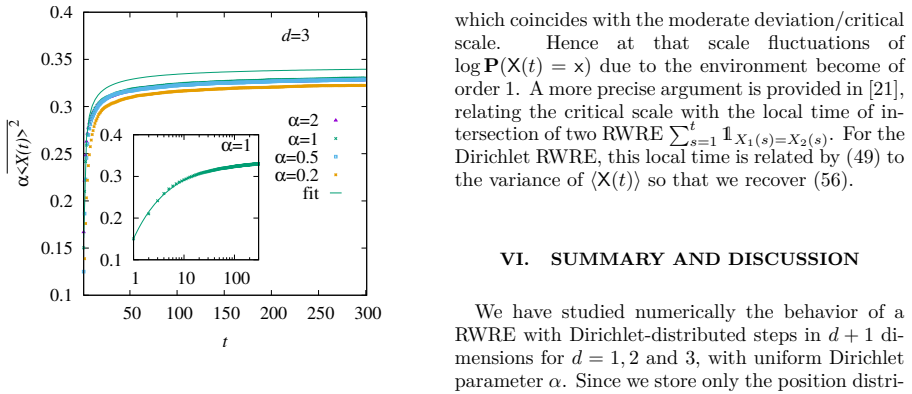
- The exact asymptotics of ⟨X(t)⟩² in d=1,2,3 match the numerics and identify its prefactor with the extreme diffusion coefficient via the local time of the difference of two Brownian motions.
Reading between the lines
- If the geometric local-time splitting used for the second moment can be made rigorous, the same two-replica machinery should yield the full weak-disorder limit distribution of Z_t, including the tail exponent μ(v) as a function of v.
- The exact relation between ⟨X(t)⟩² and the extreme diffusion coefficient suggests a practical probe: in other random-environment models, measuring this variance could locate the critical or moderate-deviation scale, including the predicted exp(C/v²) scale in d=2.
- The edge-direction behavior — a lower-dimensional subspace with its own KPZ exponent — could serve as a cleaner numerical signature of KPZ universality in 2+1 and 3+1 dimensions, since boundary distributions converge faster than off-diagonal power laws.
- The resolvent/rank-one-perturbation reading of the transition hints that the threshold might be computable in closed form for special α, for example in the Haar-unitary directed-wave representation where the model is exactly unitary, giving a lattice analogue of the bound-state condition.
Editorial analysis
A structured set of objections, weighed in public.
Referee Report
Summary. The paper studies a discrete-time random walk in a space-time i.i.d. Dirichlet random environment in dimension d+1, focusing on d=1,2,3. The authors verify numerically that the variance of log P(X(t)=tu) grows like the KPZ roughness exponent t^{2β} for off-diagonal directions, and that along the diagonal it converges to a constant determined by the stationary measure. In d=3 they claim numerical evidence for a weak-to-strong disorder transition as the direction u moves away from the diagonal, and they obtain a quantitative lower bound v_c ≥ 0.639 (k_c ≥ 11.1) from an exact two-replica second-moment calculation. They also compute exactly the sample-to-sample variance of the thermal average ⟨X(t)⟩ and relate it to the extreme diffusion coefficient. The paper combines exact stationary-measure arguments, local limit theorem asymptotics, and extensive Monte Carlo simulations.
Significance. If the main claims hold, the paper provides one of the first systematic numerical tests of the KPZ-universality conjecture for RWRE in d>1, and it gives an explicit, potentially exact handle on the d=3 transition through a second-moment calculation. The stationary-measure construction and the exact formula for the variance of ⟨X(t)⟩ are valuable independent contributions. The d=1,2 numerical results are consistent with the KPZ exponents, and the d=1 boundary case reproduces the predicted linear growth. However, the most quantitative new result — the finite second-moment formula m_2(v) and the threshold v_2 ≈ 0.639 — rests on an unproved conditional local-time decomposition in Appendix B.3.a, and the d=3 numerical 'confirmation' of the transition is based on relatively short runs. These issues need to be addressed before the claims can be regarded as fully established.
major comments (4)
- [Appendix B.3.a, Eqs. (B20)–(B23), (B37), (B45)–(B47)] The derivation of the finite second-moment formula and Table I relies on the assertion that the total intersection local time of Y, conditioned on Y(t)=0, is distributed as the sum of two independent copies of the unconditioned geometric local time with parameter R(a). The text only gives a 'roughly speaking' last-exit argument and cites Erdős–Taylor for the unconditioned local time only. If the pre-return and post-return excursions are correlated or size-biased, the conditioned law is not the independent two-copy form, and Eqs. (B37), (B45)–(B47) and all m_2(k) values in Table I would change. The pole condition of the second moment is more robust because Remark B.2 gives an independent resolvent/Sherman–Morrison route to the same threshold L(a)=(d+1)α/(d v^2), but the quantitative m_2(v) formula is not proven as written. Please provide a proof of the conditional decomposition, or at lea
- [Section IV.B, Table I and text after Eq. (44)] Table I reports simulation estimates for m_2(k) up to k=11 and claims reasonable agreement for small k, but for k≥9 the values deviate strongly from the theory (e.g., k=10: 11(1) vs 34.2218; k=11: 23(6) vs 4639.45). The authors acknowledge in the text that the tail is not sufficiently sampled to recover the theoretical values, yet the table lists these as 'Simulation' without marking them as not converged. This is misleading, and it weakens the empirical support for the exact formula near the threshold. The agreement for k≤7 is good, but the table should clearly distinguish converged estimates from upper/lower bounds or unreliable tail-limited estimates.
- [Section III.C.3 and Fig. 6] The d=3 numerical evidence for a phase transition is based on fitting Var log P(tu) to a + b t^δ for t ≤ 300, with a single inset showing δ(k) and no error bars on the variance curves. For k=13, the visible increase may be a finite-time crossover rather than asymptotic t^{2β} growth; the expected critical scale in d=3 is exponentially large in 1/v^2, so t_max=300 is very short. The authors themselves state they cannot verify the expected power law with β≈0.184. Thus the numerical 'confirmation' of the transition is not yet independent evidence; the exact second-moment lower bound is the solid result. I recommend either extending the runs, providing a more controlled finite-size analysis, or making the exploratory nature of this part explicit.
- [Section III.C.2, Fig. 4] For d=2 the claim that the off-diagonal variance is compatible with t^{2β}, β=0.2398, is supported only by the visual alignment of the data with a t^{2β} line over t≤1000, with no error bars on the variance curves and no reported fit range or uncertainty on the exponent. Since the reader is told that different power laws cannot be ruled out, the statement should be quantitative: report the fitted exponent and its confidence interval, or explicitly label the result as a consistency check rather than a measurement of β.
minor comments (5)
- [Eq. (41) and Eq. (B47)] The displayed expression for lim Z_t^2 in Eq. (41) and the second equality in Eq. (B47) appear algebraically inconsistent with the preceding formula (B46). For example, the right-hand side as typeset does not reduce to 4α(4α+1)/(4α−3v^2L(a))^2 except in special cases. Please correct the typo and check all related formulas.
- [Eq. (B1)] The definition of Z_t^2 is ambiguous: the numerator should presumably be the disorder average of the squared quenched probability, i.e., the second moment, but the notation does not clearly distinguish the disorder expectation from the quenched probability. Please clarify the overline notation in this equation and in the surrounding text.
- [Throughout] There are several typographical errors and OCR artifacts: 'damples' for 'samples' (Section III.C.2), 'orginin' for 'origin' (Section I.B), 'taxis' for 'time axis' (Section I.B), and a missing space in 'i.e.the' (Section I.B). A careful proofread is needed.
- [Fig. 5] The x-axis label in the right inset, 'x=logP(ut)−1', is confusing; it should indicate the normalized variable or explain the shift. Also, the skewness fit in Eq. (38) has many parameters for the available time range; the reported γ∞=0.26(10) has a large uncertainty and should be presented as a weak consistency check rather than a strong TW verification.
- [Section V.B, Fig. 11] The d=2 fit to the theory line required an arbitrary vertical shift of 0.27. The authors explain this, but it would strengthen the presentation to show the unshifted data as well, or to derive the expected subleading constant, so the reader can see how much of the discrepancy is captured by the asymptotics.
Circularity Check
No significant circularity: the exact formulas are derived from the model's own stationary measure and compared with independent KPZ benchmarks.
full rationale
The paper's derivation chain is self-contained rather than circular. The central exact results—the diagonal variance limit ψ′((d+1)α) (Eqs. 26–28), the two-replica second moment (Eqs. B45–B47), and the sample-to-sample thermal variance Eq. (47)—are obtained by combining the Dirichlet transition probabilities with an explicit product-form stationary measure derived in Section II, local CLT results [24], and Fourier/resolvent computations (App. B). No fitted simulation parameter is inserted into these formulas; Table I compares independent theory with simulations, and the table values are not used to build the formula. The d=1,2 variance-growth claim (Eq. 32) is calibrated against external, non-author KPZ exponents (β=1/3; β=0.2398 from [33]; β=0.184 from [34]), and the d=3 phase-transition interpretation is not forced by a self-citation: although [4] shares an author, the paper's own numerical data and exact second-moment lower bound (42) provide the evidence, and [21] (independent) mathematically supports the critical-scale picture. The only weak point the manuscript itself flags is the heuristic conditioned-local-time decomposition in App. B.3.a ('roughly speaking...'), which is an unproved probabilistic step and a correctness risk, not a circular reduction to the target claim. Consequently no step reduces to its input by construction.
Assumptions & free parameters
free parameters (3)
- d=3 variance growth exponent δ(k) =
≈0 for k<10; >0 for k≥13 (a+bt^δ fit, Fig. 6 inset)
- heavy-tail exponent μ(k) =
2.1(1) at k=11; 1.8(1) at k=12
- asymptotic limiting second moment m_2(k) =
1.2513(2), 1.401(2), 1.776(3), 2.51(2), 3.75(4), 7.4(7), 11(1), 23(6) for k=4..11
assumptions (5)
- domain assumption Atypical-trajectory log-probabilities for fixed direction u are described by the KPZ/directed-polymer universality class with the same exponents as 1+d-dimensional DP, as conjectured in [4] and partially supported by [21].
- ad hoc to paper The two-replica difference walk's total intersection local time, conditioned on return at time t, is the sum of two independent unconditioned geometric local times with common parameter R(a).
- ad hoc to paper The biased two-walk stationary measure has the product form with multiplicative weight e^{g(a)} on the diagonal (Eqs. B39–B43), via a skew-detailed-balance identity for ν.
- domain assumption In weak disorder, the normalized point-to-point probability Z_∞ has a power-law tail with exponent μ(v), and at criticality μ(v_c)=1+2/d=5/3, taken from the directed-polymer literature [42].
- domain assumption The environment is i.i.d. Dirichlet with equal parameter α across sites and directions.
Cite this review
Pith. "Pith review of Random walks in Dirichlet random environment in dimension $d+1$." pith.science (2026). https://pith.science/paper/53ITWG56
@misc{pith2026260720279,
  author       = {Pith},
  title        = {Pith review of: Random walks in Dirichlet random environment in dimension $d+1$},
  year         = {2026},
  howpublished = {\url{https://pith.science/paper/53ITWG56}},
  note         = {Machine review of arXiv:2607.20279}
}
abstract
The atypical behaviour of random walks in time-dependent random environment was recently related to Kardar-Parisi-Zhang (KPZ) growth. While this is now well-understood in spatial dimension $d=1$, further efforts are necessary to better understand these connections in dimensions $d>1$. In this paper, we study this problem numerically for $d=1, 2$ and $3$, focusing on a discrete model with Dirichlet distributed transition probabilities. This model is a generalization of an integrable model in $d=1$, and it has the advantage of admitting an explicit, product-form, stationary measure. We verify that the growth of the variance of the logarithm of point-to-point probabilities, namely from the origin to position $x$ in time $t$, is compatible with KPZ growth in dimension $d=1$ and $d=2$. In spatial dimension $d=3$, we confirm the existence of a phase transition as the angle $\vert x\vert /t$ increases and we obtain a lower bound based on an exact second moment calculation. We find that in the weak disorder phase the point-to-point probability acquires a heavy tailed distribution, and that in the strong disorder phase the cumulants of its logarithm grow with time. Further, we show that for this model, we can compute exactly the sample to sample variance of the thermal average $\overline{ \langle x \rangle^2}$ and that it is related to the extreme diffusion coefficient introduced recently.
Figures


Figures from the paper (8 more)



Reference graph
Works this paper leans on
-
[21]
consider the smoothed out field I(v,t) = ∫ φ(x)C(v,t,x)P(X(t) =tv+t 1/2x)dx (14) 3 for smooth functionsφand some appropriate deter- ministic functionC(v,t,x) (see [21, Definition 1.10]). The normalizing function is chosen so that I(v,t)−−−→ t→∞ ∫ φ(x)e −x2 2 √ 2πdx.(15) In other terms, the normalizing constant is chosen so that C(v,t,x)P(X(t) =tv+t 1/2x) ...
-
[1]
ifγ∼Gamma(α ◦) andp∼Dir(α 1,...,α d+1) are independent, then (p 1γ,...,p d+1γ) are in- dependent Gamma variables with parameters α1,...,α d+1 [31]
-
[2]
Moreover in general dimensiond, the random walk satisfies a local central limit theorem [24]
the sum of independent gamma variables with parametersα i is a Gamma random variable with parameterα◦. Moreover in general dimensiond, the random walk satisfies a local central limit theorem [24]. Combined with the knowledge of the stationary measure, this implies that whenx=O( √ t) andtgoes to infinity, P(X(t) =x)∼ e− xT D−1 x 2t (2πt)d/2 √ ˆdetD γx α◦ ,...
-
[3]
At least one of theu i is zero
Boundary cases. At least one of theu i is zero. Concretely, we may choose vectorsuof the form u= (k−d k , 1 k,..., 1 k ) (30) parameterized by somek∈[d,+∞]. The typical direction corresponds tok=d+ 1. The extreme casesk=dandk= +∞are boundary cases, which, ford⩾2 behave differently. A. Theoretical prediction In typical directions, we expect to see the vari...
-
[4]
As a consequence, it was predicted that for anyv̸= 0 ind= 2, and forv >v c ind= 3, the fluctuations of logP(X(t) =tv) scale ast β at larget, whereβis the DP exponent in dimensiond
that the fluctuations ofP(X(t) =tv) are related, as ind= 1, to those of the partition function of a continuum directed polymers with noise variance of orderv 2 =∥v∥ 2. As a consequence, it was predicted that for anyv̸= 0 ind= 2, and forv >v c ind= 3, the fluctuations of logP(X(t) =tv) scale ast β at larget, whereβis the DP exponent in dimensiond. Furtherm...
-
[5]
Typical directions (n/t≈d= ( 1 d+1,..., 1 d+1)), i.e.,along the diagonal
-
[6]
The vectoru∈(R +)d+1 is chosen so thatu 1 + ···+u d+1 = 1,u̸=d
Generic atypical directions (n=tu,u̸=d). The vectoru∈(R +)d+1 is chosen so thatu 1 + ···+u d+1 = 1,u̸=d. We also assume thatu is not be on the boundary of the simplex (that isu i∈(0,1) for all 1⩽i⩽d+ 1 but it cannot be 0 or 1)
-
[7]
Corwin and Y
I. Corwin and Y. Gu, J. Stat. Phys.166, 150 (2017)
2017
Show all 70 references
-
[8]
3 for four vec- tors: the diagonalu=d= (1/2,1/2), off diagonal vectorsu= (2/3,1/3),u= (10/11,1/11) and an edge (1,0)
Dimensiond= 1 Ford= 1 results are shown in Fig. 3 for four vec- tors: the diagonalu=d= (1/2,1/2), off diagonal vectorsu= (2/3,1/3),u= (10/11,1/11) and an edge (1,0). The results were obtained forα= 0.5, a maximum timet max = 5000 and averaged over 104 samples. For the diagonal...
-
[9]
Dimensiond= 2 The corresponding results ford= 2 andα= 0.5, witht max = 1000 and with an average over 10 4 damples are shown in Fig. 4. Here the results for the vectorsu= (1/3,1/3,1/3),u= (2/4,1/4,1/4), u= (4/6,1/6,1/6),u= (10/12,1/12,1/12) and the edgeu= (1,0,0) are shown. For...
2000
-
[10]
Our results are shown in Fig
Dimensiond= 3 Ford= 3 it is expected that there is a range of vectorsuclose to the diagonal, where var(log(P(ut)) does not increase with timet. Our results are shown in Fig. 6 for vectorsu(k) = (k−3,1,1,1)/k (k >3). One observes that for a small angle, u= (2,1,1,1)/5, the vari...
2000
-
[11]
Parekh, arXiv:2401.06073 (2024)
S. Parekh, arXiv:2401.06073 (2024)
2024
-
[12]
The sec- ond moment (Zt)2 is shown in Fig
Second moment and distribution ofZ ∞ We have sampled the probabilitiesP(ut) for lat- tice vectorsu(k) = ((k−3),1,1,1)/kand maximum timet max = 100, for 5×10 5 time series. The sec- ond moment (Zt)2 is shown in Fig. 7. It increases towards an apparent limiting value which we es...
-
[13]
(36) and (37), both shown in Fig
Third cumulant and skewness We now consider the third cumulant and the skew- ness of logP(n) as defined in Eqs. (36) and (37), both shown in Fig. 9. We have considered the cased= 3, α= 1 and maximum timet max = 300. We start at the diagonalu=d, which corresponds tok= 4. In the...
-
[14]
Kardar, G
M. Kardar, G. Parisi, and Y.-C. Zhang, Phys. Rev. Lett.56, 889 (1986)
1986
-
[15]
Barraquand and I
G. Barraquand and I. Corwin, Probability Theory and Related Fields167, 1057 (2017)
2017
-
[16]
C. A. Tracy and H. Widom, Comm. Math. Phys. 159, 151 (1994)
1994
-
[17]
Le Doussal and T
P. Le Doussal and T. Thiery, Phys. Rev. E96, 010102 (2017)
2017
-
[18]
Thiery and P
T. Thiery and P. Le Doussal, Journal of Physics A: Mathematical and Theoretical50, 045001 (2016)
2016
-
[19]
Barraquand and P
G. Barraquand and P. Le Doussal, Journal of Physics A: Mathematical and Theoretical53, 215002 (2020)
2020
- [20]
-
[22]
Barraquand and M
G. Barraquand and M. Rychnovsky, Electron. J. Probab.25, 52 (2020), id/No 119, arXiv:1905.10280
2020 arXiv
-
[23]
S. Das, H. Drillick, and S. Parekh, Probability The- ory and Related Fields , 1 (2024)
2024
-
[24]
S. Das, H. Drillick, and S. Parekh, J. Funct. Anal. 287, 90 (2024), id/No 110609, 2304.14279
2024 arXiv
- [25]
-
[26]
J. B. Hass, A. N. Carroll-Godfrey, I. Corwin, and E. I. Corwin, Physical Review E107, L022101 (2023)
2023
-
[27]
J. B. Hass, H. Drillick, I. Corwin, and E. I. Corwin, Phys. Rev. Lett.133, 267102 (2024)
2024
-
[28]
J. B. Hass, I. Corwin, and E. I. Corwin, Phys. Rev. E109, 054101 (2024)
2024
-
[29]
Hass, arXiv preprint arXiv:2505.01533 (2025)
J. Hass, arXiv preprint arXiv:2505.01533 (2025)
2025 arXiv
-
[30]
J. Hass, H. Drillick, I. Corwin, and E. Corwin, arXiv preprint arXiv:2504.00266 (2025)
2025 arXiv
-
[31]
Monthus and T
C. Monthus and T. Garel, Phys. Rev. E74, 011101 (2006)
2006
-
[32]
Junk and H
S. Junk and H. Lacoin, arXiv preprint arXiv:2402.02562 (2024)
2024
-
[33]
Pagnani and G
A. Pagnani and G. Parisi, Physical Review E92, 010101 (2015)
2015
-
[34]
Drillick and S
H. Drillick and S. Parekh, preprint (2025), arxiv:2510.22155 [math.PR]
2025
-
[35]
F. Ark, J. B. Hass, and E. I. Corwin, arXiv preprint arXiv:2508.15999 (2025)
2025 arXiv
-
[36]
Rassoul-Agha and T
F. Rassoul-Agha and T. Sepp¨ al¨ ainen, Probability theory and related fields133, 299 (2005)
2005
-
[37]
Boldrighini, R
C. Boldrighini, R. Minlos, and A. Pellegrinotti, Probability theory and related fields109, 245 (1997)
1997
-
[38]
Rassoul-Agha, T
F. Rassoul-Agha, T. Sepp¨ al¨ ainen, and A. Yilmaz, Comm. Pure Appl. Math.66, 202 (2013), 1104.3110
2013 arXiv
-
[39]
Korotkikh, Probability Theory and Related Fields184, 493 (2022)
S. Korotkikh, Probability Theory and Related Fields184, 493 (2022)
2022
-
[40]
Krajenbrink and P
A. Krajenbrink and P. Le Doussal, Physical Review E107, 014137 (2023), arXiv:2204.04720
2023 arXiv
-
[41]
A. K. Hartmann, A. Krajenbrink, and P. Le Dous- sal, Physical Review E109, 024122 (2024), arXiv:2307.15041
2024 arXiv
-
[42]
(see also [19, 20, 44]), we expect that this limit distribution has a power law tail with exponent µ(vc) = 1 + 2/d, i.e.,µ(v c) = 5/3 whend= 3. Next, we consider the third cumulant, because we expect that there exist a critical angleθ c such that for anglesθ=∠(d,u) between the...
-
[43]
The symbol≍means that both sides are of the same order ast→∞, up to constants prefactors which, in the second line, may depend onv
-
[44]
Barraquand and M
G. Barraquand and M. Rychnovsky, Communica- tions in Mathematical Physics398, 823 (2023)
2023
-
[45]
J. E. Mosimann, Biometrika49, 65 (1962)
1962
-
[46]
L. Saul, M. Kardar, and N. Read, Physical Review A45, 8859 (1992)
1992
-
[47]
´Odor, B
G. ´Odor, B. Liedke, and K.-H. Heinig, Physical 15 Review E81, 031112 (2010)
2010
-
[48]
A. K. Hartmann,Big Practical Guide to Computer Simulations(World Scientific, Singapore, 2015)
2015
-
[49]
Forster, D
D. Forster, D. R. Nelson, and M. J. Stephen, Phys. Rev. A16, 732 (1977)
1977
-
[50]
D. A. Huse, C. L. Henley, and D. S. Fisher, Phys. Rev. Lett.55, 2924 (1985)
1985
-
[51]
J. Baik, P. Deift, and K. Johansson, J. Amer. Math. Soc.12, 1119 (1999)
1999
-
[52]
Marinari, A
E. Marinari, A. Pagnani, and G. Parisi, J. Physics A: Math. Gener.33, 8181 (2000)
2000
-
[53]
A. K. Hartmann, P. L. Doussal, S. N. Majumdar, A. Rosso, and G. Schehr, Europhys. Lett.121, 67004 (2018)
2018
-
[54]
A. K. Hartmann, SciPost Phys. Lect. Notes , 100 (2025)
2025
- [55]
-
[56]
Meerson, P
B. Meerson, P. V. Sasorov, and A. Vilenkin, Journal of Statistical Mechanics: Theory and Experiment 2018, 053201 (2018)
2018
-
[57]
Lacoin, arXiv preprint arXiv:2505.13382 (2025)
H. Lacoin, arXiv preprint arXiv:2505.13382 (2025)
2025 arXiv
-
[58]
Halpin-Healy, Physical Review E—Statistical, Nonlinear, and Soft Matter Physics88, 042118 (2013)
T. Halpin-Healy, Physical Review E—Statistical, Nonlinear, and Soft Matter Physics88, 042118 (2013)
2013
-
[59]
Friedberg and Y.-K
R. Friedberg and Y.-K. Yu, Physical Review E49, 5755 (1994)
1994
-
[60]
In references [14, 17], the diffusion coefficients are defined with an extra factor 1/2 which has no effect on the definition ofλ ext
-
[61]
A. K. Hartmann, DARE data repositiory of Univer- sity of Oldenburg (2026), DOI:10.57782/G0HPXH
2026 doi
-
[62]
Erdos and S
P. Erdos and S. J. Taylor, Acta Math. Acad. Sci. Hungar11, 137 (1960)
1960
-
[63]
Appendix A: Sample to sample variance of the thermal average In this section, we explain how to obtain the estimate (47) for the sample to sample variance of the thermal average
It is unique, up to a multiplicative constant, see [21, Theorem 4.10]. Appendix A: Sample to sample variance of the thermal average In this section, we explain how to obtain the estimate (47) for the sample to sample variance of the thermal average
-
[64]
Consider two random walksX 1(t),X 2(t) in the same environment
Dimension1 Recall thatd= (1/2,1/2) denotes the diagonal direction. Consider two random walksX 1(t),X 2(t) in the same environment. The walks make steps in the directions s1 = 1 2(1,−1),s 2 = 1 2(−1,1). Sinces 1·s 1 = 1 2 ands 1·s 2 = −1 2 , we have ⟨X1(t)·X 2(t)⟩= t−1∑ s=0 P(X...
-
[65]
Dimension2 In dimensiond= 2, walks make stepse 1,e 2,e 3 inZ d+1. In the planeT 2 orthogonal to the diagonal directiond= (1/3,1/3,1/3), the random walk steps are s1 =e 1−d= 1 3(2,−1,−1),s 2 =e 2−d= 1 3(−1,2,−1),s 3 =e 3−d= 1 3(−1,−1,2).(A12) We haves i·si = 2/3 ands i·si =−1/3...
-
[66]
Dimension3 In dimensiond= 3, the random walk steps in the hyperplaneT 3 orthogonal todare s1 = 1 4(3,−1,−1,−1),s 2 = 1 4(−1,3,−1,−1),s 3 = 1 4(−1,−1,3,−1),s 4 = 1 4(−1,−1,−1,3) so that the covariance of increments when walks start from the same point is s1·s 1q+s 1·s 2(1−q) = ...
-
[67]
In order to arrive at the pointvts 1, the walk must makessteps towardss 1 andt−ssteps in other directions, withss 1·s 1 +(t−s)s 1·s 2 =vts 1·s 1
First moment Let us start with the computation of the first moment P(X(t) =tvs 1). In order to arrive at the pointvts 1, the walk must makessteps towardss 1 andt−ssteps in other directions, withss 1·s 1 +(t−s)s 1·s 2 =vts 1·s 1. Sinces 1.s2 = −1 d+1, we obtain that s=t 1 +vd d...
-
[68]
Second moment Now we use the fact that P(X(t) =x) 2 =P(X 1(t) =X 2(t) =x) where the couple of random walks (X1,X 2) has transition probabilities P(X1(t) =x 1 +si,X 2(t) =x 2 +sj ⏐⏐⏐X1(t−1) =x 1,X 2(t−1) =x 2) = { pi pj ifx 1̸=x 2, pipj ifx 1 =x 2. (B8) In the notations above, ...
-
[69]
Analysis of the local time As in the theorem of Erd¨ os-Taylor [49], astgoes to infinity, in dimensiond⩾3, we will show that the local time∑t−1 u=0 1˜X1(u)=˜X2(u) converges to a geometric random variable, and we need to determine its parameter. By decomposing the trajectory of...
-
[70]
From [42] (see also [19, 20, 44] ) we expect that this limit distribution has a power law tail with exponentµ(v)>µ(v c) = 1 + 2/d, i.e.,µ(vc) = 5/3 ind= 3
Limit in the weak disorder phase In the weak disorder phase we expect that the distribution of the random variableP(X(t) =vts 1) converges to a limit fort→+∞. From [42] (see also [19, 20, 44] ) we expect that this limit distribution has a power law tail with exponentµ(v)>µ(v c...
Reviewed August 1, 2026 · model on record in the stance chip above.
Discussion (0). Sign in to comment.