Pith. sign in

REVIEW 2 major objections 5 minor 3 references

Generative Visual Communication in the Era of Vision-Language Models

T0 review · 2 major / 5 minor · reviewed 2026-08-12 · deepseek-v4-flash

Pith's one-line read This dissertation claims that pretrained vision-language models, constrained to vector outputs and guided by task-specific regularizations, can automatically produce effective visual communication designs across sketches, typography…

desk verdict A PhD thesis that reprints five strong, well-evaluated papers; no new research results, but the compiled work is coherent and the human studies carry the evidence despite the CLIP-circularity concern. read the letter →

arxiv 2411.18727 v1 pith:5FHEAG7P submitted 2024-11-27 cs.CV cs.AI

classification cs.CVcs.AI
keywords visualcommunicationvision-languagemodelssketchabstractionsemantictypographyword-as-imagetext-to-videoanimationconceptdecompositionvectorgraphics
verification ladder T0 review T1 audit T2 compute T3 formal

The pith

A machine-rendered reading of the paper's core claim, the machinery that carries it, and where it could break.

The reading

This dissertation argues that pretrained vision-language models can be turned into practical tools for visual communication by restricting the output to editable vector graphics and adding task-specific regularizations. The claim is demonstrated in four settings: object and scene sketching with controllable abstraction, typographic word-as-image illustrations, text-driven animation of static sketches, and hierarchical decomposition of visual concepts for design inspiration. If the claim holds, designers gain initial solutions in editable form, namely vector files with Bézier strokes or letter outlines, that can be refined by hand without needing task-specific sketch or illustration datasets. The central mechanism is the same across all four settings: a frozen pretrained model supplies semantic guidance, and a differentiable rasterizer channels that guidance into the parameters of vector strokes.

What carries the argument

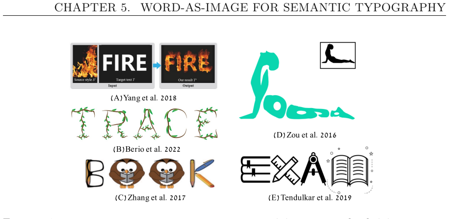
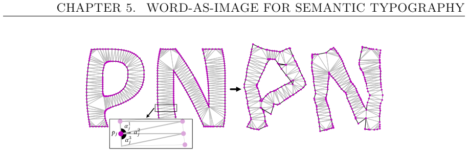
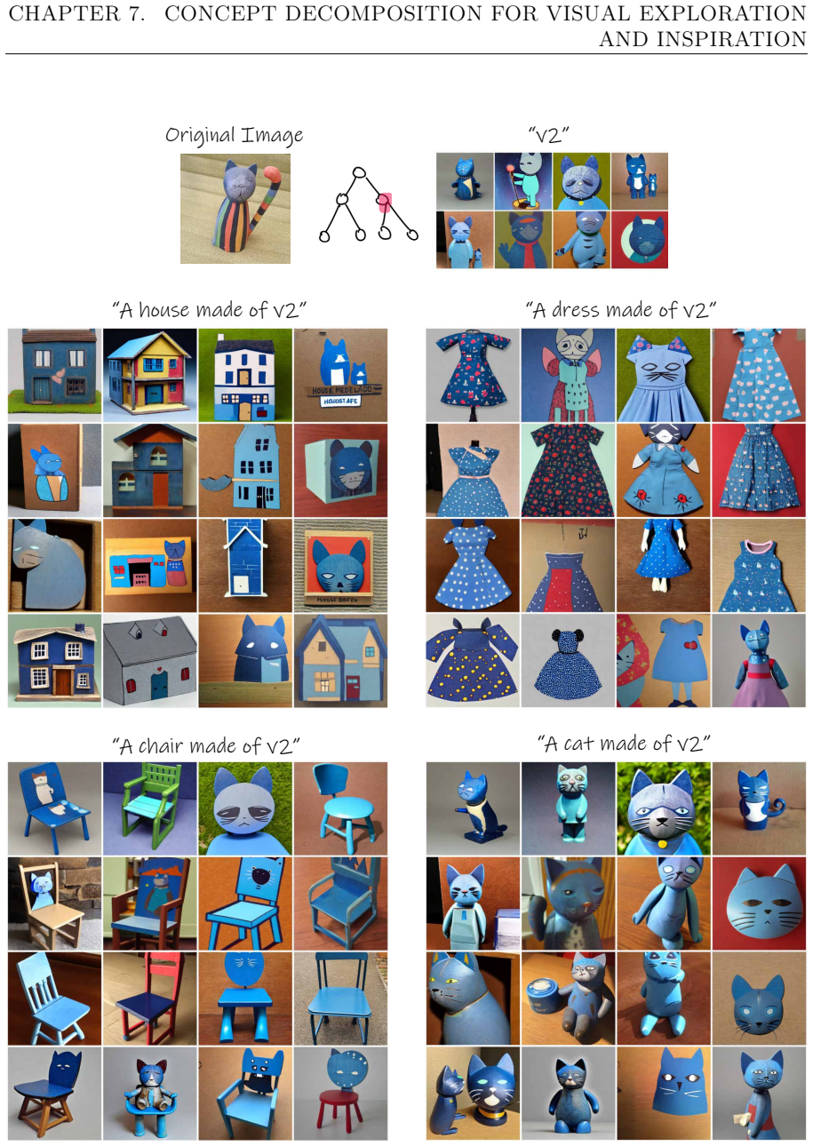
The load-bearing object is the frozen vision-language prior: CLIP's shared image-text embedding space for sketches, and the diffusion-model distribution captured by Stable Diffusion and text-to-video models for typography, animation, and inspiration. The connection to editable design output is made by a differentiable rasterizer that turns Bézier control points into pixels, so that semantic losses can be backpropagated directly into stroke or letter parameters. Three regularizers carry the domain-specific constraints: an as-conformal-as-possible deformation and a tone-preservation loss keep deformed letters legible and on-font; a learned stroke-probability vector with a sparsity loss produces smooth simplification along the simplicity axis; and a neural displacement field split into local and global motion predicts per-frame offsets that animate strokes while preserving the sketch's identity. For concept decomposition, the mechanism is a learned embedding vector per tree node that is injected into the text-to-image model's latent space and optimized to reconstruct the parent concept from its children.

What would settle it

Run the CLIPasso pipeline on a simple MNIST digit such as "3" with four or sixteen strokes: if the resulting strokes merely trace the digit's edges and cannot be recognized as a three by human viewers, the claim that CLIP's prior transfers semantic meaning to sparse vector renderings is falsified for that input class.

Watch

Extended reading notes

Core claim

On the paper's own terms, the central discovery is that the semantic-visual knowledge inside pretrained vision-language models can substitute for human-drawn datasets in generative design tasks. CLIPasso and CLIPascene show that optimizing Bézier strokes under a CLIP-based loss produces recognizable object and scene sketches at multiple abstraction levels, where abstraction is controlled by stroke count or by two disentangled axes, fidelity and simplicity. Word-as-Image shows that deforming the vector outline of letters under a score-distillation loss from Stable Diffusion, with conformal and tone-preserving regularizers, yields legible typography that visually expresses a word's meaning. Breathing Life Into Sketches shows that a pretrained text-to-video model, again via score distillation sampling, can drive a neural displacement field that moves existing sketch strokes according to a text prompt. Concept Decomposition shows that textual-inversion-style embeddings can be optimized into a tree of sub-concepts that reconstruct a parent concept and recombine across concepts. The unifying claim is that large pretrained priors, combined with a differentiable vector renderer and domain-specific losses, are sufficient to generate concise, effective visual communication.

Load-bearing premise

The entire program assumes that CLIP and Stable Diffusion, trained mostly on natural images, align well enough with sparse black-and-white vector renderings that gradient descent against their embeddings yields human-meaningful abstraction; the thesis itself shows this assumption breaking on inputs like MNIST digits.

Editorial extensions

If this is right

  • Designers can obtain editable vector sketches of arbitrary objects or scenes, with abstraction level set by stroke count or by the fidelity and simplicity axes.
  • Word-as-image typography can be generated automatically while keeping letters legible and the original font recognizable, producing usable logo and poster starting points.
  • Static sketches can be turned into short vector animations by writing a text prompt, removing the need for skeletal rigs or reference motion capture.
  • Visual inspiration can be structured: a concept can be decomposed into a tree of aspects, and aspects from different concepts can be recombined to generate novel designs.
  • Because none of the tools requires task-specific datasets, the same algorithmic recipe can be applied to new categories and input types without retraining.

Reading between the lines

Editorial extensions of the paper, not claims the author makes directly.

  • Inference: the same constrained-optimization recipe, a frozen vision-language prior plus differentiable vector renderer plus structure regularizers, is likely portable to other design artifacts such as icons, pictograms, charts, and motion graphics, since the losses are not specific to the four studied mediums.
  • Inference: as vision-language models improve their alignment on non-photographic renderings, the documented failure modes on digits and fine-grained attributes should shrink without any algorithmic change, which is a direct testable prediction.
  • Inference: the fidelity and simplicity axes of CLIPascene offer a quantitative, controllable definition of "abstraction" that could be reused as a parameter in other generative design tools, letting users dial a visual from literal to iconic.
  • Inference: combining the letter-deformation idea with the animation framework would yield semantic kinetic typography, where words deform into their meaning and then move, an extension that follows naturally from the dissertation's stated goal of editable, vector-based visual communication.
Share X Bluesky LinkedIn Reddit HN

Editorial analysis

A structured set of objections, weighed in public.

Desk editor's note, referee report, and a circularity audit.

Referee Report

2 major / 5 minor

Summary. This PhD dissertation investigates whether pretrained vision-language models (VLMs) such as CLIP, Stable Diffusion, and text-to-video models can automatically generate effective visual communication designs. The thesis is organized around four research directions: object and scene sketching with controllable abstraction (CLIPasso and CLIPascene), semantic typography in the form of word-as-image illustrations, text-driven animation of static sketches, and hierarchical concept decomposition for visual inspiration. Each chapter presents an optimization-based method that produces editable vector representations, guided by CLIP or diffusion-model priors, and includes qualitative results, comparisons to prior work, and human or automatic evaluations. The central claim is that these pretrained priors can be leveraged to simplify complex ideas into clear, concise, vector-based visuals that support designers' creative workflows.

Significance. If the claims hold, the dissertation makes a strong and timely contribution: it demonstrates that general-purpose vision-language priors, not task-specific sketch or typography datasets, can drive a range of design-oriented generative tasks while preserving vector editability. The individual methods have already been published in top venues (SIGGRAPH, ICCV, CVPR), several with best-paper or honorable-mention awards, and the thesis provides a coherent framing around visual communication. Strengths include the explicit use of human perceptual studies in every chapter, the honest documentation of failure modes inherited from CLIP (e.g., MNIST digits and fine-grained attributes in Fig. 3.17), and the release of project pages with code and results. The main risk is that some quantitative evaluations rely on CLIP-family metrics that share the same pretrained priors as the optimization objectives, so they do not independently measure human-perceived effectiveness; the human studies, while genuine, are narrow in coverage.

major comments (2)
  1. [§3.3.3 (Table 3.3), §4.3.3 (Table 4.2), §6.3 (Table 6.1)] The zero-shot CLIP classifiers used to measure sketch and video recognizability operate in the same embedding family as the losses being optimized (Eq. 3.3 with CLIP ResNet101; Eq. 4.2 with CLIP-ViT; and the SDS loss in Chapter 6 with text-to-video priors). Consequently, high quantitative scores may partially reflect the optimizer's success at satisfying CLIP's internally consistent representation rather than independent human-perceived effectiveness. The human studies are a genuine safeguard, but they are limited in breadth: 5 animal classes and 25 images in the CLIPasso perceptual study, 30 images in the CLIPascene user study, 10 letters in the Word-as-Image study, and a preference study for animation. To make the quantitative evaluations load-bearing for the thesis's central claim, the author should either provide a per-item calibration of CLIP scores against human judgments (e.g., correlation or confusion analysis by abstraction level) or explicitly label CLIP-based metrics as proxies and rest the effectiveness claim primarily on the human studies. Without this, statements such as 'we validate that our sketches accurately depict the input object' are stronger than the evidence supports.
  2. [§4.2.3 (Eq. 4.5–4.7)] The 'perceptually smooth simplification' of the simplicity axis is achieved by sampling the loss-ratio factor r exponentially, justified by appeal to the Weber-Fechner law. No perceptual experiment is reported to confirm that the resulting simplification steps are perceptually uniform for sketch abstraction; Figure 4.9 shows only two anecdotal sequences. Since the simplicity axis is a core claimed contribution of CLIPascene, the smoothness claim should be validated with a user study or softened to 'heuristically smooth' in the text.
minor comments (5)
  1. [Global] There are multiple typos and formatting inconsistencies: 'resterized' in the Figure 3.4 caption, 'interpertable' in Section 3.1, 'A viv University' on the title page, 'on the painting the cars' in the Figure 3.17b caption, and generally inconsistent hyphenation and spacing throughout the compiled text.
  2. [§3.3.3] In Table 3.3, the 'Human Sketches' baseline should be more precisely defined; it is not clear whether these are the human sketches from SketchyCOCO or from another source, and how they were selected.
  3. [§4.3.3] The CLIP zero-shot classification in Table 4.2 uses a set of 200 class names, but the source of this set is not specified, and the criterion 'at least 2 of the top 5 classes' should be justified or reported alongside alternative thresholds.
  4. [Notation] The thesis uses different CLIP variants (ResNet101, ViT-B/32, ViT-B/16) across chapters without a unified notation table; this makes it harder to track which pretrained model is used for optimization versus evaluation in each chapter.
  5. [§5.3.1] The Word-as-Image perceptual study in Table 5.1 is based on only 10 letters; while the qualitative results on 50 words are extensive, the quantitative claim of 'very high' concept recognizability should be qualified by the small sample size and the large standard deviations reported.

Circularity Check

3 steps flagged · score 4.0 of 10

CLIP-based evaluation metrics partially re-measure the optimization objective, but independent human studies keep the central claims non-circular.

  1. other [Section 3.3.3 (Quantitative Evaluation), Eq. (3.3) and Table 3.3]
    "and a CLIP ViT-B/32 zero-shot classifier using text prompts defined as "A sketch of a(n)class-name". Note that this is not the CLIP model we use for training."

    The optimization objective (Eq. 3.3) minimizes Lsemantic = dist(CLIP(I), CLIP(R({si}))), a cosine distance in CLIP embedding space. The CLIP ViT-B/32 zero-shot classifier then scores the sketch by the closeness of the same family of CLIP embedding to class text embeddings. A sketch driven toward the image's CLIP embedding is statistically forced to be classified by a CLIP model as the same class, so the CLIP column of Table 3.3 largely re-measures the training objective rather than providing independent evidence of human recognizability. The paper's human perceptual study (Table 3.2) is independent and mitigates this, so the circularity is partial.

  2. other [Section 4.3.3 (Quantitative Evaluation), Eq. (4.2) and Table 4.2]
    "Using a pre-trained ViT-B/16 CLIP model (different than the one used for training), we performed zero-shot image classification over each input image and the corresponding resulting sketches from the different methods."

    Training guides sketches with LCLIP(S, I, ℓk) = ||CLIP_l(S) − CLIP_l(I)||^2 (Eq. 4.2). Recognizability in Table 4.2 is then measured by zero-shot classification with a CLIP ViT-B/16 model, i.e., by whether the sketch's CLIP embedding is close to the input image's CLIP embedding and to class text embeddings. The evaluation therefore inherits the same embedding geometry that the loss optimizes; high scores partly reflect optimization success rather than human perception. The accompanying user study (Table 4.3) is an independent check and supports the central claim, so this is not a load-bearing circularity.

1 more flagged steps
  1. other [Section 6.3 (Results), Table 6.1]
    "Quantitative metrics. (a) CLIP-based consistency and text-video alignment comparisons to open-source image-to-video baselines. (b) The same CLIP-metrics used for an ablation study."

    The sketch animation is optimized with a score-distillation loss from a pretrained text-to-video diffusion model (Sec. 6.2.2), and the quantitative evaluation uses CLIP-based text-video alignment. Both rely on vision-language embedding similarities, so the metric is a partial re-measurement of the guiding prior rather than a fully independent test. The user study (Fig. 6.8) provides external evidence for the central claim, and the CLIP metric is secondary, so this is a minor issue.

full rationale

The dissertation is a compilation of five published methods, each built as an optimization against a frozen pretrained VLM (CLIP or Stable Diffusion). The derivations themselves are not circular: the losses (Eqs. 3.3, 4.2, 5.3, and the SDS losses in Chs. 5–6) define objectives, and the outputs are produced by optimization rather than by definition. The main circularity risk is confined to quantitative evaluation: the CLIP-based recognition and alignment scores in Chs. 3, 4, and 6 use the same family of embedding geometry as the training losses, so those tables partly re-measure the optimization objective rather than providing fully independent confirmation. However, the central claims are also supported by human perceptual studies (Tables 3.2, 4.3, 5.1; Fig. 6.8) and by qualitative comparisons to external baselines, so the methods are not forced by their inputs. Self-citations (e.g., CLIPasso as the basis of CLIPascene) are normal incremental extensions and are not used as an unverified uniqueness argument. Overall, there is partial evaluation circularity but no load-bearing derivation circularity, giving a score of 4.

Assumptions & free parameters 6 free parameters · 5 assumptions · 0 invented entities

The thesis depends on the alignment quality of pretrained vision-language models (CLIP, Stable Diffusion) as a semantic prior for vector rendering optimization. These are external, unproven resources. Hyperparameters are numerous but standard; none are fitted to a target world constant. There are no invented physical or conceptual entities.

free parameters (6)
  • ws semantic loss weight (CLIPasso) = 0.1
    Eq. 3.3; balances geometric and semantic CLIP distances; chosen by hand, affects abstraction results.
  • CLIP geometric layers (CLIPasso) = layers 3 and 4 of ResNet101 CLIP
    Used in Eq. 3.2; intermediate activation layers chosen by hand to capture geometry.
  • CLIP-ViT fidelity layers (CLIPascene) = {2, 7, 8, 11}
    Section 4.2.2; separate MLP trained per layer to realize the fidelity axis; layer selection is a design choice.
  • Initial stroke count (CLIPascene) = 64
    Section 4.2.2; fixed number of Bezier strokes before simplification; the simplicity axis is then learned.
  • alpha ACAP weight (Word-as-Image) = 0.5
    Eq. 5.3; weight of the conformal deformation loss; set by hand and claimed to work across words and fonts.
  • beta_t schedule (Word-as-Image) = a=100, b=300, c=30
    Eq. 5.4; Gaussian weight schedule for the tone loss; tuned to allow semantic deformation before tone preservation activates.
assumptions (5)
  • domain assumption CLIP embeddings capture semantic similarity between natural images and abstract vector sketches
    Section 2.3 and used in CLIPasso (Eq. 3.1-3.3) and CLIPascene (Eq. 4.2). If false, optimization would not produce recognizable abstractions.
  • domain assumption Score distillation sampling (SDS) gradients from Stable Diffusion provide a meaningful signal for optimizing vector parameters
    Section 2.5; used in Word-as-Image (Eq. 5.3) and Breathing Life into Sketches. Relies on the pretrained text-to-image prior.
  • standard math Differentiable rasterization (DiffVG) yields usable gradients for Bezier control point optimization
    Section 2.1; foundational tool assumption, verified by prior work [150].
  • ad hoc to paper The Weber-Fechner law justifies exponential sampling of simplification factors for perceptually smooth abstraction
    Section 4.2.3; used to define r_j^k factors in CLIPascene; a perceptual-psychology assumption imported to justify a design choice.
  • domain assumption U2-Net and LaMa provide sufficiently accurate foreground/background separation and inpainting for scene sketching
    Section 4.2.4; if segmentation fails, foreground/background sketch decomposition is harmed.

how reviews work

0 comments
Cite this review

Pith. "Pith review of Generative Visual Communication in the Era of Vision-Language Models." pith.science (2026). https://pith.science/paper/5FHEAG7P

@misc{pith2026241118727,
  author       = {Pith},
  title        = {Pith review of: Generative Visual Communication in the Era of Vision-Language Models},
  year         = {2026},
  howpublished = {\url{https://pith.science/paper/5FHEAG7P}},
  note         = {Machine review of arXiv:2411.18727}
}
read the original abstract

Visual communication, dating back to prehistoric cave paintings, is the use of visual elements to convey ideas and information. In today's visually saturated world, effective design demands an understanding of graphic design principles, visual storytelling, human psychology, and the ability to distill complex information into clear visuals. This dissertation explores how recent advancements in vision-language models (VLMs) can be leveraged to automate the creation of effective visual communication designs. Although generative models have made great progress in generating images from text, they still struggle to simplify complex ideas into clear, abstract visuals and are constrained by pixel-based outputs, which lack flexibility for many design tasks. To address these challenges, we constrain the models' operational space and introduce task-specific regularizations. We explore various aspects of visual communication, namely, sketches and visual abstraction, typography, animation, and visual inspiration.

Figures

Figures reproduced from arXiv: 2411.18727 by the authors.

Figure 1.1
Figure 1.1. Historical visual communication. (a) Cave paintings (Cantabia Spain) were the first form of visual communication. They originate to around 40,000 years ago. (b) An ancient Sumerian tablet with one of the first personal signatures in the world. (c) Egyptian hieroglyphics developed from Sumerian Cuneiform script, where images and symbols create a visual language. While the term ’visual communication’ encompasses a bro… view at source ↗
Figure 1.2
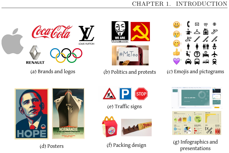
Figure 1.2. Examples of modern visual communication designs across many mediums. Motivated by the fundamental role of visual communication in our society, in this dissertation we aim to explore the ability of computers to automatically produce effec￾tive visual communication designs across different mediums, especially in light of recent advancements in large vision-language models and generative models (also called “Gen￾erativ… view at source ↗
Figure 1.3
Figure 1.3. Text-to-image generation examples. These examples were created completely au￾tomatically by feeding the written text into DallE2 [212]. A significant research effort in the computer vision and graphics communities aims at enhancing VLMs in terms of generation quality [200, 222], speed [234, 237, 162], and better user control [306, 40, 50, 186]. In addition, it has been discussed that such models hold immense potenti… view at source ↗
Figures from the paper (106 more)
Figure 1.4
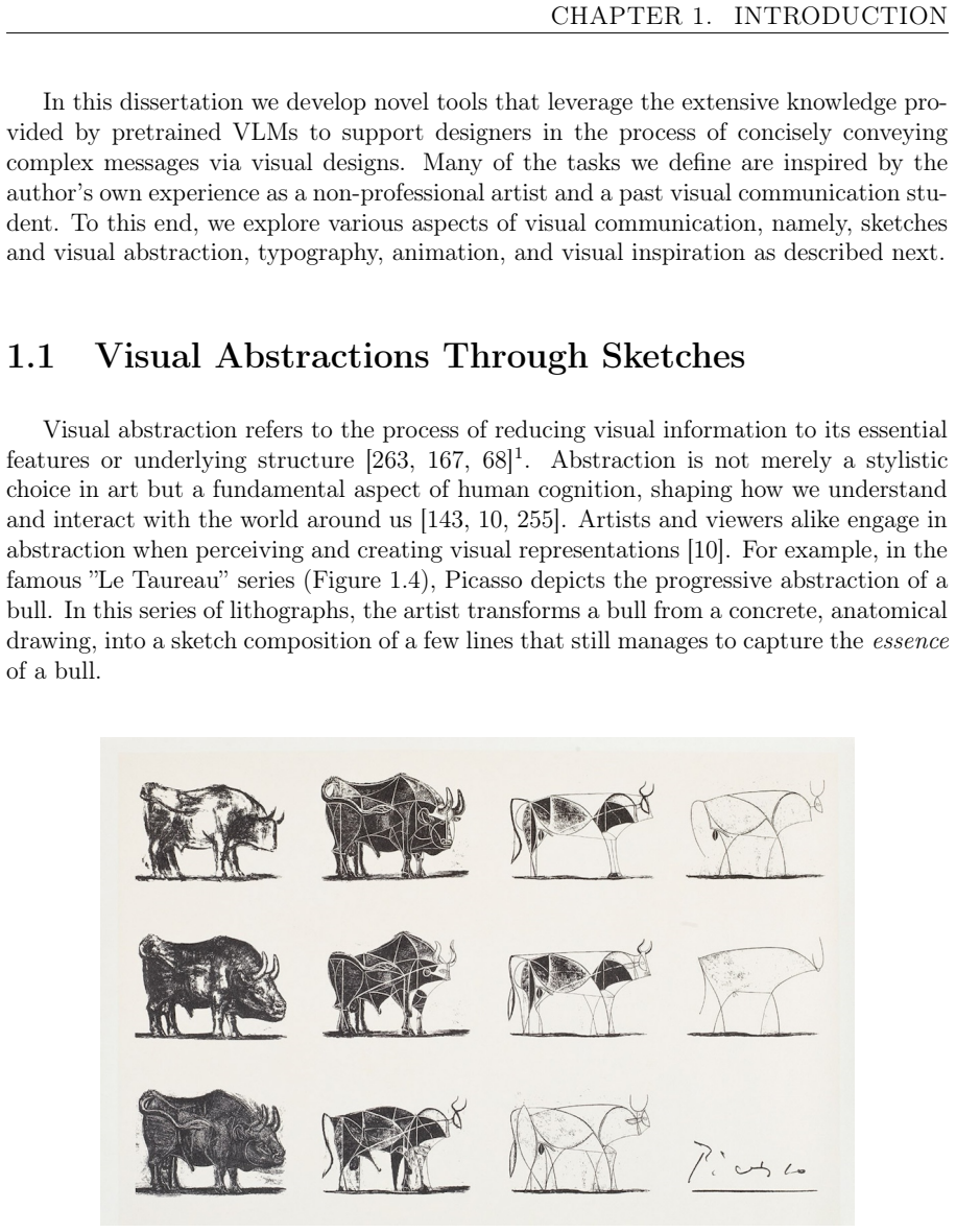
Figure 1.4. Figure 1.4: “Le Taureau” by Picasso — note how the abstraction process is achieved by gradually removing elements while the bull’s essence is preserved. 1This is the definition of “visual abstraction” in the context of visual communication and in the context of this dissertation…
Figure 1.5
Figure 1.5. Figure 1.5: (1) A sketch by Vincent Van Gogh for his famous piece “Chair”. (2) The Citibank logo, designed by Paula Scher, started with a sketch on a napkin during one of her first meetings with the company. (3) Drawings by Leonardo Da Vinici on the mechanical powers and forces.…
Figure 1.6
Figure 1.6. Figure 1.6: Examples of iconic visual communication designs that leverage typographical el￾ements in creative and strategic ways to convey messages effectively. (a) The Public Theatre advertisement posters, designed by Scher, 1994. (b) DADA book cover by Paul Rand, 1951. (c) Pos…
Figure 1.7
Figure 1.7. Figure 1.7: Examples of word-as-image illustrations made by the artist Ji Lee [146]. Designing word-as-image illustrations presents several challenges, primarily due to the need to integrate typography with visual imagery effectively, while maintaining legibility. In addition, c…
Figure 1.8
Figure 1.8. Figure 1.8: "La Linea", a classic Italian animated series created by Osvaldo Cavandoli in the 1960s. Italian animated series created by Osvaldo Cavandoli in the 1960s (see fig. 1.8). It features a character simply known as "The Line," a simple outline character who encounters va…
Figure 1.9
Figure 1.9. Figure 1.9: Examples of design inspired by visual concepts taken from other concepts. (a) top left - fashion design by Iris Van Herpen and Chair by Emmanuel Touraine inspired by nature patterns, bottom left - the Lotus Temple in India, inspired by the lotus flower (b) Beijing Na…
Figure 2.1
Figure 2.1. Figure 2.1: Illustration of a vector image. The bird is composed of a set of shapes (shown at the bottom). Additionally, we illustrate the difference between a raster representation on a pixel grid, and a vector representation which is resolution free. Scalable Vector Graphics (…
Figure 2.2
Figure 2.2. Figure 2.2: Illustration of Bézier curves of degrees 1 to 4 (left to right) and how they are constructed recursively based on t ∈ [0, 1]. 28 [PITH_FULL_IMAGE:figures/full_fig_p031_2_2.png]
Figure 2.3
Figure 2.3. Figure 2.3: An example of a dataset composed of images of cats. This group of images can be thought of as discrete samples from a distribution over the pixel space that defines all possible cat images. A generative model is tasked with generating new images that belong to this d…
Figure 2
Figure 2. Figure 2: (the illustration was taken from the CLIP paper [210]). [PITH_FULL_IMAGE:figures/full_fig_p033_2.png]
Figure 2.4
Figure 2.4. Figure 2.4: CLIP jointly trains an image encoder and a text encoder to predict the correct pairings of a batch of (image, text) training examples. The illustration was taken from the CLIP paper [210]. Being trained on a wide variety of image domains along with lingual concepts, …
Figure 2.5
Figure 2.5. Figure 2.5: A visualization of forward diffusion process and reverse denoising process of an image. Chain of length T. For image synthesis, the most successful models rely on a reweighted variant of the variational lower bound on p(x), which mirrors denoising score-matching [85]…
Figure 3.1
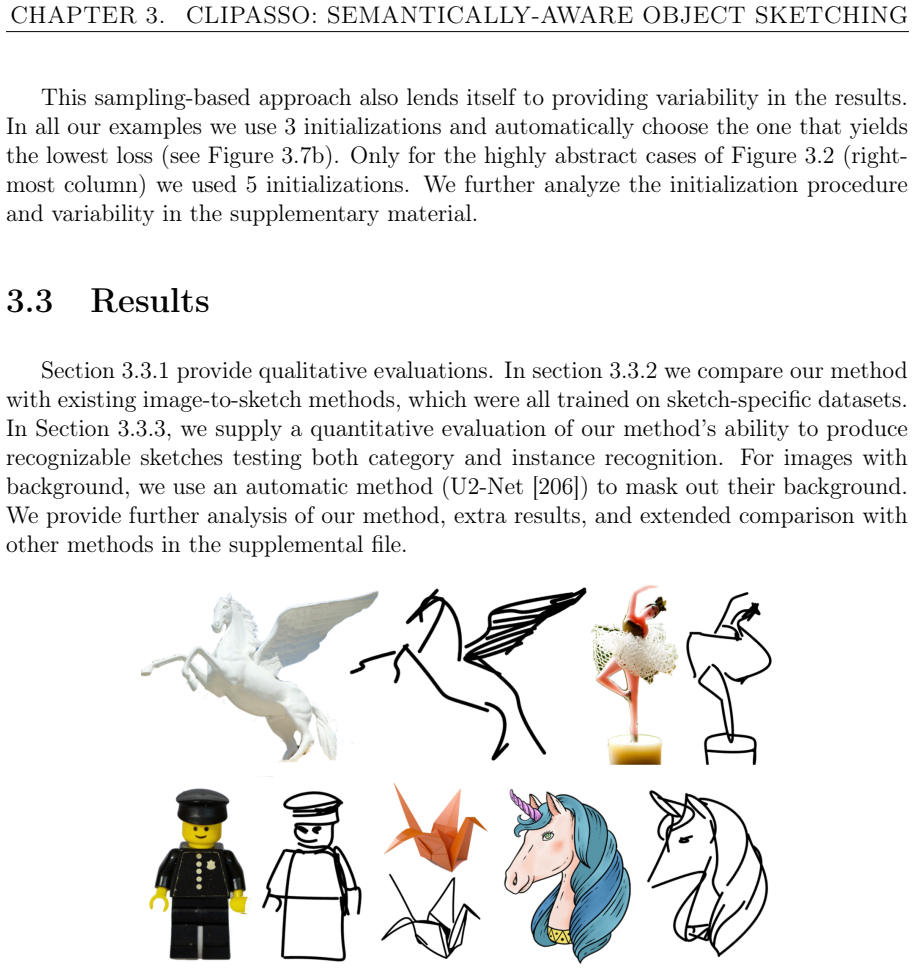
Figure 3.1. Figure 3.1: Our work converts an image of an object to a sketch, allowing for varying levels of abstraction, while preserving its key visual features. Even with a very minimal representation (the rightmost flamingo and horse are drawn with only a few strokes), one can recognize …
Figure 3.2
Figure 3.2. Figure 3.2: Different levels of abstraction produced by our method. Left to right: input images and increased level of abstraction. The top three sketches were produced using 16, 8, and 4 strokes in columns 2, 3, and 4, respectively, and the man’s sketch was produced using 32, 1…
Figure 3.3
Figure 3.3. Figure 3.3: Variations in style and abstraction among sketch datasets — examples are ar [PITH_FULL_IMAGE:figures/full_fig_p042_3_3.png]
Figure 3.4
Figure 3.4. Figure 3.4: Method overview – Given a target image I, and the number of strokes n, a saliency map is used as the distribution to sample the initial strokes locations {s1, ..sn}. A differentiable rasterizer R is used to create a resterized sketch S. Both the sketch and the image …
Figure 3.5
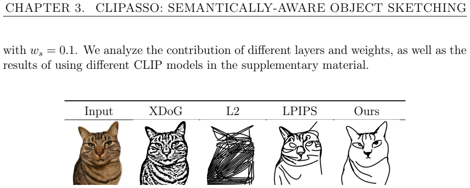
Figure 3.5. Figure 3.5: Loss functions comparison — we optimize the strokes by minimizing different losses: L2 loss simply encourages the filling of colored pixels, LPIPS is more semantically aware, but the resulting sketch is still close to the edge map (see the XDog edges for comparison).…
Figure 3.6
Figure 3.6. Figure 3.6: The sketch appearance throughout the optimization iterations. ©Face image from [184], used with permission. 43 [PITH_FULL_IMAGE:figures/full_fig_p046_3_6.png]
Figure 3.7
Figure 3.7. Figure 3.7: Strokes Initialization. (a) Left to right: input, the saliency map produced from CLIP ViT activations, final distribution map (adjusted to adhere to image edges) with sampled initial stroke locations (in red), the sketch produced using the proposed initialization pro…
Figure 3
Figure 3. Figure 3: a illustrates this procedure. It can be seen that our saliency-based initial [PITH_FULL_IMAGE:figures/full_fig_p047_3.png]
Figure 3.8
Figure 3.8. Figure 3.8: Sketches produced by our method for infrequent categories. 3.3.1 Qualitative Evaluation Our approach is different from conventional sketching methods in that it does not utilize a sketch dataset for training, rather it is optimized under the guidance of CLIP. Thus, o…
Figure 3.9
Figure 3.9. Figure 3.9: Changing sketch style. (a) From left to right are the results produced by our method when using Bézier curves with 4, 3, and 2 control points (cp), respectively. We can see how this affects the style of the output sketch. (b) Using Adobe Illustrator, horse — pencil f…
Figure 3.10
Figure 3.10. Figure 3.10: Levels of Abstraction Comparison — in the top and left part are comparisons to Muhammad et al. [187]. The leftmost column shows the input image, and the next four columns show different levels of abstraction. For the shoe and chair our results were produced using 32…
Figure 3.11
Figure 3.11. Figure 3.11: Comparison to Existing Image-to-Sketch Works — the leftmost column shows the input images. The methods presented are (A) Kampelmühler and Pinz [124], (B) Li et al. [152], (C) Li et al. [148] (D) Song et al. [235], (E) SketchLattice [204]. Input CLIPDraw Ours Input C…
Figure 3.12
Figure 3.12. Figure 3.12: Comparison to CLIPDraw [72]. All sketches were produced using 16 strokes. In [PITH_FULL_IMAGE:figures/full_fig_p051_3_12.png]
Figure 3.13
Figure 3.13. Figure 3.13: Confusion matrices of category-level recognition of the perceptual study of our method with four and eight strokes (left and middle matrices) and the method of Kampelmühler and Pinz [124]. and Pinz [124]. The three matrices show that the majority of the classificati…
Figure 3.14
Figure 3.14. Figure 3.14: A visualisation of the appearance of the mean sketch µs (the larger giraffes) at two levels of abstraction, next to six samples of distinct sketches from the corresponding set. We also compare the diversity of the sketches generated by our method to the ones drawn b…
Figure 3.15
Figure 3.15. Figure 3.15: Diversity score as a function of the abstraction level. 7 sketches using our method for each face and level of abstraction using 7 different seeds, each seed imitates a different artist in this case [PITH_FULL_IMAGE:figures/full_fig_p055_3_15.png]
Figure 3.16
Figure 3.16. Figure 3.16: An example of the sketches used in the diversity study. In each row, we show seven distinct sketches generated from a single input face, along with the average sketch that corresponds to this set in the rightmost column. The first two rows show the sketches drawn by…
Figure 3.17
Figure 3.17. Figure 3.17: Limitations inherited from CLIP. Figure (a) illustrates that the semantics of the input image (e.g. the digit three) are missing. This results in our method being unable to convey this meaning, which could potentially be expressed with only four strokes. Rather, as …
Figure 3.18
Figure 3.18. Figure 3.18: Results of 90 random images from 90 classes from the SketchyDatabase [PITH_FULL_IMAGE:figures/full_fig_p058_3_18.png]
Figure 3.19
Figure 3.19. Figure 3.19: Sketching "in the wild": results of 100 random images of cats from Sketchy [PITH_FULL_IMAGE:figures/full_fig_p059_3_19.png]
Figure 4.1
Figure 4.1. Figure 4.1: Our method converts a scene image into a sketch with different types and levels of abstraction by disentangling abstraction into two axes of control: fidelity and simplicity. The sketches on the left were selected from a complete matrix generated by our method (an ex…
Figure 4.2
Figure 4.2. Figure 4.2: Scene complexity. (A) contains a single, central object with a simple background, (B) contains multiple objects (the cat and vase) with a slightly more complicated background, and (C) contains both foreground and background that include many details. Our work tackles…
Figure 4.3
Figure 4.3. Figure 4.3: Drawings of different scenes by different artists. Notice the significant differences in style and level of abstraction between the drawings — moving from more detailed and precise (left) to more abstract (right). The second row shows how the level of abstraction not…
Figure 4.4
Figure 4.4. Figure 4.4: The fidelity axis. From left to right, using the same number of strokes the sketches gradually depart from the geometry of the input image, but still convey the semantics of the scene. We define two axes representing two types of abstractions and produce sketches by …
Figure 4.5
Figure 4.5. Figure 4.5: The simplicity axis. On the left, we start with a more detailed sketch and as we move to the right the sketch is gradually simplified while still remaining consistent with the overall appearance of the initial sketch [PITH_FULL_IMAGE:figures/full_fig_p063_4_5.png]
Figure 4.6
Figure 4.6. Figure 4.6: Artistic stylization of the strokes using Adobe Illustrator. fidelity and simplicity axes, as shown in [PITH_FULL_IMAGE:figures/full_fig_p063_4_6.png]
Figure 4.7
Figure 4.7. Figure 4.7: Single sketch generation scheme. In gray, we show our training scheme for producing a single sketch image at a single level of fidelity. In the bottom left we show the additional components used to generate a single sketch at a single level of simplicity. MLPloc. Thi…
Figure 4.8
Figure 4.8. Figure 4.8: Trade-off between Lsparse and LCLIP . As the sketch becomes sparser, Lsparse obtains lower score. However, the sketch also becomes less recognizable with respect to the input image, resulting in a higher penalty for LCLIP . To implement the probabilistic-based remova…
Figure 4.9
Figure 4.9. Figure 4.9: Smooth v.s. non-smooth simplification. In the first row, the simplification appears perceptually smooth, where a consistent change in the degree of abstraction is performed. The second row demonstrates a non-smooth simplification, as there is a visible “jump” between…
Figure 4.10
Figure 4.10. Figure 4.10: Iterative simplification of the sketch Sk. To produce a simplified sketch S j k we iteratively fine-tune MLPloc (blue) and MLPsimp (orange) w.r.t Lratio loss defined by each r j k . smooth transition in the first row forms an exponential relation between Lsparse and…
Figure 4.11
Figure 4.11. Figure 4.11: Scene decomposition. Top right – an example of the separation technique. Left – scene sketching results obtained with and without decomposing the scene. Bottom – examples of sketch editing by modifying the style of strokes. of [PITH_FULL_IMAGE:figures/full_fig_p071…
Figure 4.12
Figure 4.12. Figure 4.12: Sketches along the two abstraction axes. In Figures 4.1, 4.4 and 4.12 (top) we show sketch abstractions along the fidelity axis, where the sketches become less precise as we move from left to right, while still conveying the semantics of the images (for example the …
Figure 4.13
Figure 4.13. Figure 4.13: Comparison to CLIPasso [262]. Note how CLIPasso fails to capture the background in most cases, especially at higher abstraction levels, despite having the same stroke budget. The sketches produced by UPDG [301] and Chan et al. [38] are detailed, closely following th…
Figure 4.14
Figure 4.14. Figure 4.14: Scene sketching results and comparisons. From left to right are the sketches obtained using XDoG [281], UPDG [301], Photo-Sketching [149], and Chan et al. [38]. On the right, are three representative sketches produced by our method depicting three levels of abstract…
Figure 4.15
Figure 4.15. Figure 4.15: Example of how images were pre￾sented to participants in the user study. To make a fair comparison, we com￾pared the methods which produce ab￾stract sketches (CLIPasso [262] and Photo-Sketching [149]) with our more abstract sketches (highest abstraction level of our…
Figure 4.16
Figure 4.16. Figure 4.16: The 4×4 matrix of sketches produced by our method. Columns from left to right illustrate the change in fidelity, from precise to loose, and rows from top to bottom illustrate the visual simplification. 75 [PITH_FULL_IMAGE:figures/full_fig_p078_4_16.png]
Figure 4.17
Figure 4.17. Figure 4.17: The 4×4 matrix of sketches produced by our method. Columns from left to right illustrate the change in fidelity, from precise to loose, and rows from top to bottom illustrate the visual simplification. 76 [PITH_FULL_IMAGE:figures/full_fig_p079_4_17.png]
Figure 4.18
Figure 4.18. Figure 4.18: The 4×4 matrix of sketches produced by our method. Columns from left to right illustrate the change in fidelity, from precise to loose, and rows from top to bottom illustrate the visual simplification. 77 [PITH_FULL_IMAGE:figures/full_fig_p080_4_18.png]
Figure 4.19
Figure 4.19. Figure 4.19: The 4×4 matrix of sketches produced by our method. Columns from left to right illustrate the change in fidelity, from precise to loose, and rows from top to bottom illustrate the visual simplification. 78 [PITH_FULL_IMAGE:figures/full_fig_p081_4_19.png]
Figure 4.20
Figure 4.20. Figure 4.20: The 4×4 matrix of sketches produced by our method. Columns from left to right illustrate the change in fidelity, from precise to loose, and rows from top to bottom illustrate the visual simplification. 79 [PITH_FULL_IMAGE:figures/full_fig_p082_4_20.png]
Figure 5.1
Figure 5.1. Figure 5.1: A few examples of our word-as-image illustrations in various fonts and for different textual concept. The semantically adjusted letters are created completely automatically using our method, and can then be used for further creative design as we illustrate here.1 Sem…
Figure 5.2
Figure 5.2. Figure 5.2: Manually created word-as-image illustrations [PITH_FULL_IMAGE:figures/full_fig_p085_5_2.png]
Figure 5.3
Figure 5.3. Figure 5.3: More word-as-images produced by our method. Note how styles of different fonts are preserved by the semantic modification. 5.1 Related Work Text Stylization One approach to text stylization is artistic text style transfer, where the style from a given source image is…
Figure 5.4
Figure 5.4. Figure 5.4: Examples of previous text stylization works – (A) Yang et al. [298], (B) Berio et al. [21], (C) Zhang et al. [305], (D) Zou et al. [319], and (E) Tendulkar et al. [243]. Most use color and texture or copy icons onto the letters. Our work concentrates on subtle geomet…
Figure 5.5
Figure 5.5. Figure 5.5: Illustration of the letter’s outline and control points before (left) and after (right) the subdivision process. The orange dots are the initial Bézier curve segment endpoints. The blue dots are the remaining control points respectively before and after subdivision. …
Figure 5
Figure 5. Figure 5: ). We analyse the effect of the number of control points in Section 5.3.3. [PITH_FULL_IMAGE:figures/full_fig_p088_5.png]
Figure 5.6
Figure 5.6. Figure 5.6: An overview of our method. Given an input letter li represented by a set of control points P, and a concept (shown in purple), we optimize the new positions Pˆ of the deformed letter ˆli iteratively using three loss functions together (marked as 1-3). At each iterati…
Figure 5.7
Figure 5.7. Figure 5.7: Visual illustration of the constraint Delaunay triangulation applied to the initial shapes (left) and the resulting ones (right), for the word “pants”. The ACAP loss maintains the structure of the letter after the deformation. The zoomed rectangle shows the angles fo…
Figure 5.8
Figure 5.8. Figure 5.8: Our tone-preserving loss preserves the local tone of the font by comparing the low-pass filter of the letters images before (left) and after deformation (right). It constrains the adjusted letter not to deviate too much from the original. This example is of the lette…
Figure 5.9
Figure 5.9. Figure 5.9: Word-as-images produced by our method for the word “YOGA”, using eight different fonts. Tone Preservation Loss To preserve the style of the font as well as the structure of the letter we add a local-tone preservation loss term. This term constrains the tone (amount o…
Figure 5.10
Figure 5.10. Figure 5.10: Additional examples of word-as-image applied on Chinese characters. In Chinese, a whole word can be represented by one character. From left: bird, rabbit, cat and surfing (two last characters together). The complexity of characters imposes an additional challenge fo…
Figure 5.11
Figure 5.11. Figure 5.11: Comparison to alternative methods based on large scale text-to-image models. On the left are the letters used as input (only for SDEdit, CLIPDraw, and ours), as well as the desired object of interest. The results from left to right obtained using Stable Diffusion [2…
Figure 5.18
Figure 5.18. Figure 5.18: The results of all letters and words are presented in the supplementary [PITH_FULL_IMAGE:figures/full_fig_p094_5_18.png]
Figure 5
Figure 5. Figure 5: illustrates the impact of the letter’s initial number of control points. [PITH_FULL_IMAGE:figures/full_fig_p095_5.png]
Figure 5.12
Figure 5.12. Figure 5.12: The effect of the initial number of control points on outputs. On the left are the input letters and the target concepts used to generate the results on the right. Po indicates the original number of control points as extracted from the font, P is the input letter w…
Figure 5.13
Figure 5.13. Figure 5.13: The effect of using only the SDS loss: note how the third row simply looks like icon illustrations, while the second row still resembles legible letters [PITH_FULL_IMAGE:figures/full_fig_p096_5_13.png]
Figure 5.14
Figure 5.14. Figure 5.14: Altering the weight α of the Lacap loss. On the leftmost column are the original letters and concepts used, then from left to right are the results obtained when using α ∈ {1, 0.75, 0.5, 0.25, 0}. "Bear" "Singer" "Giraffe" Input 1 5 30 200 Without Ltone [PITH_FULL_…
Figure 5.15
Figure 5.15. Figure 5.15: Altering the σ parameter of the low pass filter using in the Ltone loss. On the leftmost column are the original letters and concepts used, then from left to right are the results obtained when using σ ∈ {1, 5, 30, 200}, and without Ltone. 5.4 Limitations and Future…
Figure 5.16
Figure 5.16. Figure 5.16: Replacing the SDS loss with a CLIP-based loss. 95 [PITH_FULL_IMAGE:figures/full_fig_p098_5_16.png]
Figure 5.17
Figure 5.17. Figure 5.17: Failure cases: letters that do not convey the word’s concept (top), or lose their legibility (bottom – ‘C’ in ‘Coat’ and ’G’ in ’Gorilla’) [PITH_FULL_IMAGE:figures/full_fig_p099_5_17.png]
Figure 5.18
Figure 5.18. Figure 5.18: Word-as-images produced by our method. This subset was chosen from the random set of words. 96 [PITH_FULL_IMAGE:figures/full_fig_p099_5_18.png]
Figure 5.19
Figure 5.19. Figure 5.19: Additional results produced by our method. 97 [PITH_FULL_IMAGE:figures/full_fig_p100_5_19.png]
Figure 6.1
Figure 6.1. Figure 6.1: Given a still sketch in vector format and a text prompt describing a desired action, our method automatically animates the drawing with respect to the prompt.1 Sketches serve as a fundamental and intuitive tool for visual expression and commu￾nication [69, 11, 85]. S…
Figure 6.2
Figure 6.2. Figure 6.2: Data representation. Each curve (black or blue) is a cubic Bézier curve with 4 control points (red, shown for the blue curves). The total number of control points in the given sketch is denoted by N. For each frame and control point pi , we learn a displacement ∆pi (…
Figure 6.3
Figure 6.3. Figure 6.3: Text-driven optimization. At each training iteration: (1) We duplicate the initial control points across k frames and sum them with their predicted offsets. We render each frame and concatenate them to create the output video. (2) We use the SDS loss to extract a sig…
Figure 6.4
Figure 6.4. Figure 6.4: Network architecture. The input to the network is the initial set of control points Z init (left, gray), and the output is the set of displacements ∆Z. The network consists of three parts. First, each control point p j i is projected with Mshared into a latent repres…
Figure 6.5
Figure 6.5. Figure 6.5: Qualitative results. Our model converts an initial sketch and a driving prompt describing some desired motion into a short video depicting the sketch moving according to the prompt. See the supplementary for the full videos and additional results. Global path The goa…
Figure 6.6
Figure 6.6. Figure 6.6: Our method can be used to animate the same sketch according to different prompts. These are typically restricted to actions that the portrayed subject would naturally perform. See the supplementary videos for more examples. (4) Gen2 (3)VideoCrafter Ours (1) ZeroScope…
Figure 6.7
Figure 6.7. Figure 6.7: Qualitative comparisons. Image-to-video models suffer from artifacts and struggle to preserve the sketch shape (or even remain in a sketch domain). Animated drawings relies on skeletons and pre-captured reference motions. Hence, it cannot generalize to new domains. S…
Figure 6.8
Figure 6.8. Figure 6.8: User study results. We pit our full model against each ablation setup. The blue bar indicates the percent of responders that preferred our full model over each baseline. Dashed area is one standard error. Input Ours w/o network w/o global w/o local [PITH_FULL_IMAGE:…
Figure 6.9
Figure 6.9. Figure 6.9: Qualitative ablation. Removing the neural network or the global path leads to shape deviations or jittery motion due to the need for higher learning rates (see supplementary videos). Modeling only global movement improves shape consistency, but fails to create realis…
Figure 6.10
Figure 6.10. Figure 6.10: Method limitations. The method may struggle with certain sketch representations, fail to tackle multiple objects or complex scenes, or create undesired shape changes. Moreover, it is restricted to motions which the text-to-video prior can create. biases. For example…
Figure 7.1
Figure 7.1. Figure 7.1: Left: Our method provides a tree-structured visual exploration space for a given unique concept. The nodes of the tree (“vi”) are newly learned textual vector embeddings, injected to the latent space of a pretrained text-to-image model. The nodes encode different asp…
Figure 7.2
Figure 7.2. Figure 7.2: Examples of design inspired by vi￾sual concepts taken from other concepts. (a) top left - fashion design by Iris Van Herpen and Chair by Emmanuel Touraine inspired by na￾ture patterns, bottom left - the Lotus Temple in India, inspired by the lotus flower (b) Beijing …
Figure 7.3
Figure 7.3. Figure 7.3: High level pipeline of the “binary reconstruction” stage. We optimize two sibling nodes vl , vr at a time (marked in red and blue). (a) We first generate a small training set of images I p depicting the concept in the parent node using a pretrained text-to-image mode…
Figure 7.4
Figure 7.4. Figure 7.4: Optimization iterations. The embedding of both children nodes vl , vr are initilized with the word “object”. During iterations, they gradually depict two aspects of the original concept. Note that using both embedding together reconstructs the original parent concept…
Figure 7.5
Figure 7.5. Figure 7.5: We demonstrate two sets of random images generated from two different vector embeddings. An example of a consistent set can be seen on the left, where the concept depicted in the node is clear. We show an inconsistent set on the right, where images appear to depict m…
Figure 7.6
Figure 7.6. Figure 7.6: Consistency scores matrix between image sample sets of nodes. The seed selec￾tion process favors pairs of siblings that have a high consistency score within themselves, and low consistency score between each other. In this example, the left pair is better than the ri…
Figure 7.7
Figure 7.7. Figure 7.7: Examples of inter-tree combinations. We use our method to produce trees for the four concepts depicted in the first row. We then combine aspects from different trees to generate a set of inter-tree combinations (the chosen aspects are shown next to each concept). We …
Figure 7.8
Figure 7.8. Figure 7.8: Combining the learned aspects in natural sentences to produce aspect-based vari￾ations. The original concepts are shown at the top. In the third and fourth rows are our text-based generation results applied with the aspects depicted in the second row. Under “TI” we s…
Figure 7.9
Figure 7.9. Figure 7.9: Comparison of optimizing for two child nodes (left) v.s. three child nodes (right). Using three nodes increases the chance of arriving at inconsistent or irrele￾vant concepts. In terms of consistency, we observe that when optimizing more than two nodes at a time, the…
Figure 7.10
Figure 7.10. Figure 7.10: Comparing different initialization approaches. The columns show the differ [PITH_FULL_IMAGE:figures/full_fig_p129_7_10.png]
Figure 7.11
Figure 7.11. Figure 7.11: We demonstrate four general cases of decomposition failure. 128 [PITH_FULL_IMAGE:figures/full_fig_p131_7_11.png]
Figure 7.12
Figure 7.12. Figure 7.12: Exploration tree for the cat sculpture. At the bottom we show examples of possible intra-tree combinations. 129 [PITH_FULL_IMAGE:figures/full_fig_p132_7_12.png]
Figure 7.13
Figure 7.13. Figure 7.13: Exploration tree for a decorated teapot. At the bottom we show examples of possible text-based generation. 130 [PITH_FULL_IMAGE:figures/full_fig_p133_7_13.png]
Figure 7.14
Figure 7.14. Figure 7.14: More examples of inter-tree combinations. 131 [PITH_FULL_IMAGE:figures/full_fig_p134_7_14.png]
Figure 7.15
Figure 7.15. Figure 7.15: Exploration tree for the “round bird” object. At the bottom we show examples of possible intra-tree combinations and text-based generation. 132 [PITH_FULL_IMAGE:figures/full_fig_p135_7_15.png]
Figure 7.16
Figure 7.16. Figure 7.16: Exploration tree for the “scary mug” object. At the bottom we show examples of possible intra-tree combinations. 133 [PITH_FULL_IMAGE:figures/full_fig_p136_7_16.png]
Figure 7.17
Figure 7.17. Figure 7.17: Exploration tree for the “colorful teapot” object. At the bottom we show [PITH_FULL_IMAGE:figures/full_fig_p137_7_17.png]
Figure 7.18
Figure 7.18. Figure 7.18: Exploration tree for the “wooden pot” object. At the bottom we show [PITH_FULL_IMAGE:figures/full_fig_p138_7_18.png]
Figure 7.19
Figure 7.19. Figure 7.19: More examples of text based generation for the “cat sculpture” object. The [PITH_FULL_IMAGE:figures/full_fig_p139_7_19.png]
Figure 7.20
Figure 7.20. Figure 7.20: More examples of text based generation for the “cat sculpture” object. The [PITH_FULL_IMAGE:figures/full_fig_p140_7_20.png]
Figure 7.21
Figure 7.21. Figure 7.21: More examples of text based generation for the “wooden saucer bear” object. [PITH_FULL_IMAGE:figures/full_fig_p141_7_21.png]
Figure 7.22
Figure 7.22. Figure 7.22: More examples of text based generation for the “wooden saucer bear” object. [PITH_FULL_IMAGE:figures/full_fig_p142_7_22.png]

Discussion (0). Continue with ORCID to comment.

Reference graph

Works this paper leans on

3 extracted references · 2 canonical work pages

  1. [318]

    Unpaired Image- To-Image Translation Using Cycle-Consistent Adversarial Networks

    Jun-Yan Zhu, Taesung Park, Phillip Isola, and Alexei A. Efros. “Unpaired Image- To-Image Translation Using Cycle-Consistent Adversarial Networks”. In:ICCV. 2017

  2. [319]

    Legible Compact Calligrams

    Changqing Zou, Junjie Cao, Warunika Ranaweera, Ibraheem Alhashim, Ping Tan, Alla Sheffer, and Hao Zhang. “Legible Compact Calligrams”. In:ACM Transac- tions on Graphics 35.4 (July 2016), pp. 1–12. issn: 0730-0301, 1557-7368. doi: 10.1145/2897824.2925887

  3. [320]

    Shape skeletonization by identi- fying discrete local symmetries

    Ju Jia Zou, Hung-Hsin Chang, and Hong Yan. “Shape skeletonization by identi- fying discrete local symmetries”. In:Pattern Recognition34.10 (2001), pp. 1895– 1905. 168

Pith tools

Reviewed August 12, 2026 · model on record in the stance chip above.