REVIEW 4 major objections 5 minor 38 references
CycleGAN with a Blur Kernel for Deconvolution Microscopy: Optimal Transport Geometry
T0 review · 4 major / 5 minor · reviewed 2026-08-14 · deepseek-v4-flash
Pith's one-line read This paper claims that a cycleGAN with a single deep generator and a linear blur kernel performs unsupervised blind and non-blind 3D deconvolution microscopy, and that its training objective is exactly a dual optimal transport problem…
desk verdict Useful single-generator cycleGAN with a linear blur kernel for non-blind deconvolution; the blind and OT claims are thinner than the abstract suggests. read the letter →
The pith
A machine-rendered reading of the paper's core claim, the machinery that carries it, and where it could break.
The reading
What carries the argument
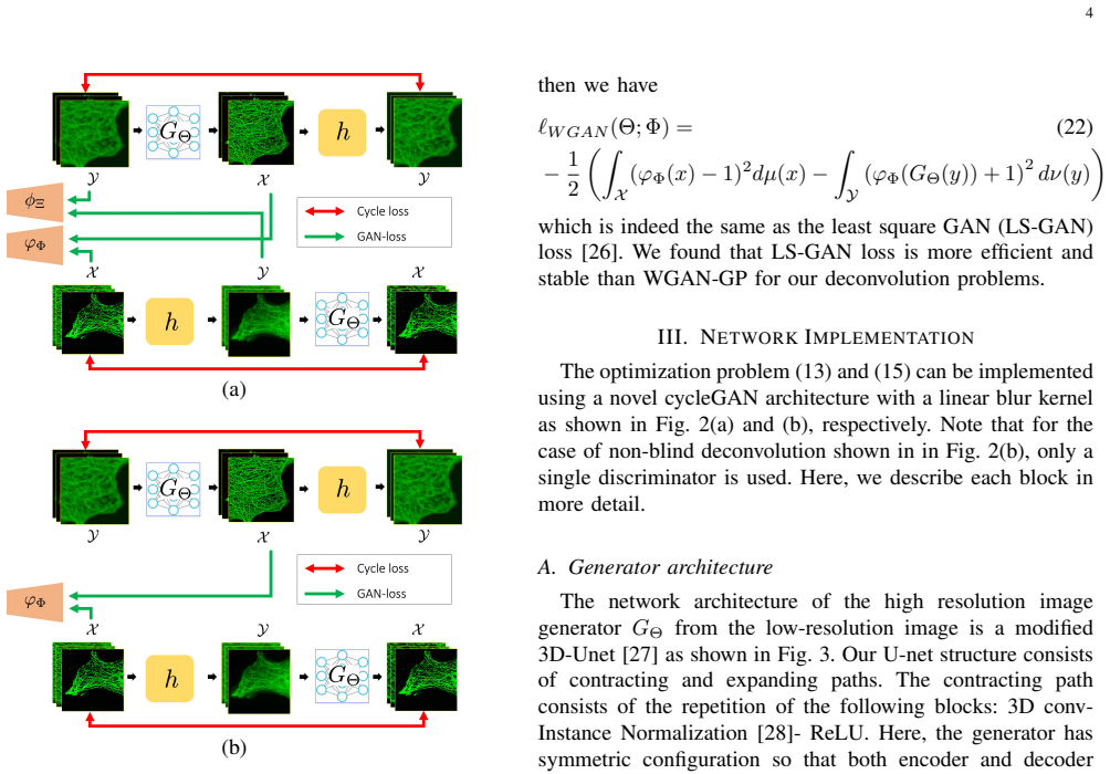
The central object is the penalized least squares transport cost c(x,y;Θ,h)=‖y−h∗x‖+‖GΘ(y)−x‖, which couples the unknown high-resolution image x, the measured blurred image y, the deep generator GΘ, and the blur kernel h. In the optimal transport formulation, this cost defines the average transportation cost between the high-resolution measure and the low-resolution measure, and its Kantorovich dual yields the cycle-consistency loss and the Wasserstein GAN discriminator losses. The linear convolution h doubles as the blur generator, so that when the global minimum is reached the map satisfies both y=h∗x and x=GΘ(y), which is exactly the desired deconvolution consistency.
What would settle it
Measure the depth-dependent PSF of a real microscope using a bead stack, train the blind network on one focal plane, and then check whether the single learned 31x31x31 kernel predicts the blur at distant z-slices within the noise level; if the predicted blur is systematically wrong along the optical axis, the single-kernel assumption fails.
Extended reading notes
Core claim
The central claim is that for deconvolution microscopy, the standard cycleGAN's two deep generators are unnecessary: a single deep generator from low-resolution to high-resolution, paired with a linear blur kernel as the low-resolution generator, suffices. The paper derives this architecture from the Kantorovich dual formulation of optimal transport, using the penalized least squares cost c(x,y;Θ,h)=‖y−h∗x‖+‖GΘ(y)−x‖ as the transport cost. The resulting objective splits into a cycle-consistency loss and adversarial discriminator losses, with the linear convolution h providing automatic data consistency. For the non-blind case, the blur kernel is fixed and only one generator-discriminator pair remains. The paper reports that this approach outperforms conventional cycleGAN on simulated and real fluorescence microscopy data and generalizes across noise levels and PSF models.
Load-bearing premise
The method's load-bearing premise is that a single space-invariant convolution kernel plus additive noise describes the microscope's entire blurring process, even though real microscope PSFs vary with depth and signal level and the paper itself reports that the learned kernel also absorbs the noise generation process.
Editorial extensions
If this is right
- A single deep generator plus a linear blur kernel can perform unsupervised blind deconvolution of 3D fluorescence volumes without paired high-resolution data.
- Replacing the blur-path deep generator with a convolution layer enforces data consistency by construction, since the generated high-resolution image must reproduce the measurement when reblurred.
- The non-blind deconvolution setting simplifies to one generator and one discriminator, and the paper reports it reconstructs more accurately than the blind setting.
- Because the architecture is derived from a dual optimal transport problem, cycle consistency is not an ad-hoc regularizer but a consequence of the PLS transport cost, giving the method a principled geometric interpretation.
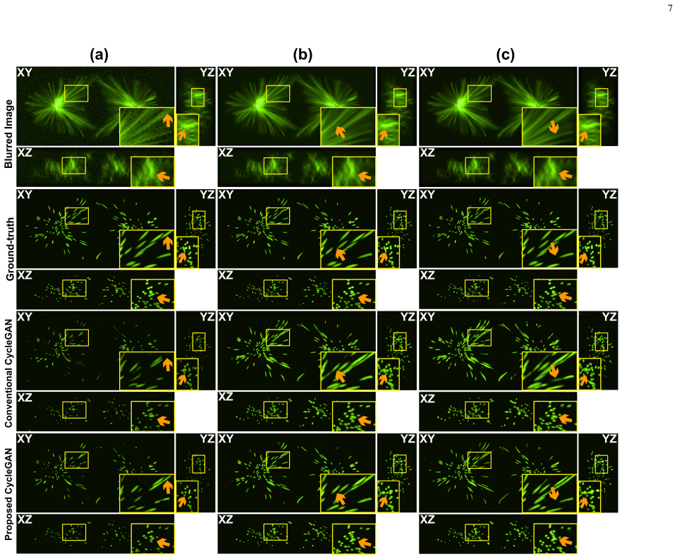
- The method generalizes to different noise levels and to a different PSF model without retraining, which the paper demonstrates with a Richards-Wolf PSF.
Reading between the lines
- The same single-generator-plus-linear-forward-model trick should transfer to other linear inverse problems, such as CT, MRI, or motion deblurring, whenever the forward operator is known or can be parameterized simply.
- Because the learned kernel also absorbs the noise generation process, as the paper itself notes, a testable extension is to model noise separately from the PSF layer, which should yield a cleaner estimate of the true point spread function.
- The unpaired-data claim still depends on the two image domains differing mainly by blur and noise; if the low-resolution domain also carries other systematic differences, cycle consistency could lock onto the wrong correspondence, so applying the method to multimodal data would require explicit modeling of those differences.
Signed reviews
Editorial analysis
A structured set of objections, weighed in public.
Referee Report
Summary. The paper proposes an unsupervised cycle-consistent GAN for 3-D deconvolution microscopy in which the low-resolution generator is replaced by a single learnable linear blur kernel, so that only one deep generator (a 3D U-Net) and one or two discriminators are trained. The authors claim that this architecture is a dual formulation of an optimal transport problem with a penalized least-squares cost, and they report experiments on synthetic microtubule data (with Born&Wolf and Richards&Wolf PSFs, several noise levels) and on real epifluorescence microscopy data, comparing against supervised baselines, conventional cycleGAN, and AutoQuant X3.
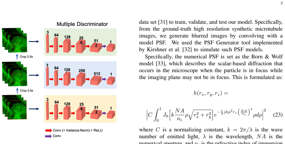
Significance. If the central claims hold, the proposed architecture is a meaningful step for unsupervised deconvolution: it reduces cycleGAN complexity, imposes physics-based data consistency through a convolutional layer, and offers an interpretable estimated PSF. The simulation study is well designed: it uses external synthetic ground truth, two PSF models, multiple SNR levels, and comparisons to supervised and conventional cycleGAN baselines, and the reported gains over conventional cycleGAN are plausible. The main weaknesses are that the OT-duality result is cited from a companion preprint rather than derived here, the actual implementation replaces the WGAN loss with an LS-GAN loss whose equivalence to the OT dual is questionable, the blind PSF estimate is acknowledged to be inaccurate in the axial direction and to absorb noise, and the real-data evaluation is circular because the training reference and the comparison baseline are both AutoQuant X3 outputs. The paper is therefore valuable but its theoretical and real-data claims require substantial additional support.
major comments (4)
- [Section II-A, Eqs. (8)-(11)] The central identity min_{Theta,H} K(Theta,H) = min_{Theta,H} max_{Phi,Xi} l(Theta,H;Phi,Xi) is stated as a result from the companion paper [23] (arXiv:1909.12116), but no derivation is given here. Since [23] is a preprint from the same group, the abstract's claim that "the proposed architecture is indeed a dual formulation of an optimal transport problem" is not substantiated within this manuscript. Please provide a self-contained proof (or a precise statement of the conditions under which the equality holds) or cite a peer-reviewed version of [23]; otherwise the theoretical contribution is only an assertion.
- [Section II-C and III-B] The OT dual formulation in Eqs. (8)-(11) requires Kantorovich potentials that are 1-Lipschitz, but the implementation uses the least-squares GAN loss, not a Wasserstein loss. The manuscript attempts to bridge this in Eqs. (19)-(22) by claiming that LS-GAN is equivalent to WGAN with a quadratic penalty. This equivalence is not established and is generally false: the LS-GAN objective is related to a Pearson chi-square-type divergence, not the Wasserstein distance. Moreover, Eq. (22) as printed has a sign error: the integrals over X and Y should be summed, not subtracted, for the claimed equivalence to hold. Since the trained objective is not the WGAN loss, the statement that the network solves the OT dual problem is not supported.
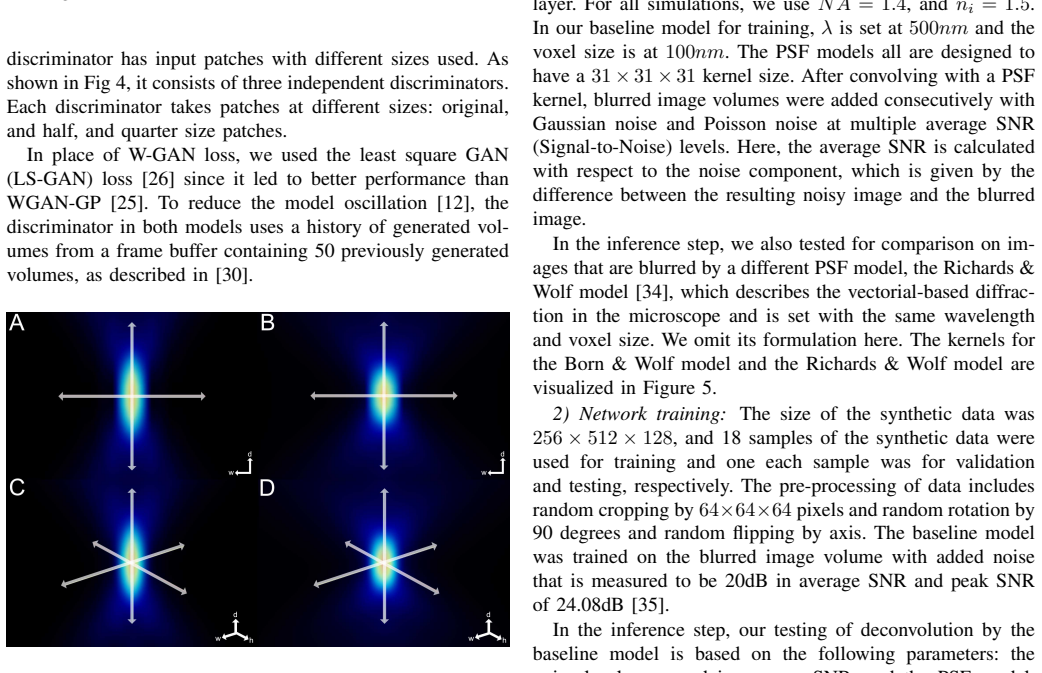
- [Section V-A.5 and Eq. (14)] The blind deconvolution model assumes a single space-invariant blur kernel h in Eq. (2) and uses one learned 31x31x31 or 20x20x20 kernel. Real fluorescence PSFs are depth-dependent and signal-dependent, so the cycle-consistency term in Eq. (14), \int ||y - h*G(y)|| dnu(y), is misspecified for real data. The authors themselves report in Section V-A.5 that the learned linear layer shows axial discrepancy and "not only learns the PSF but also noise generation processes." The simulation study validates only the fixed-PSF settings (Born&Wolf and Richards&Wolf), so the blind-deconvolution claim for real microscopy data is not supported by the evidence presented.
- [Section V-B, Fig. 12] The real-data experiment is circular: the high-resolution reference domain used for training consists of AutoQuant X3-deconvolved volumes, and the experimental comparison in Fig. 12 uses AutoQuant X3 as a baseline. The network is therefore trained to imitate AutoQuant X3 outputs, so reporting improved visual quality over AutoQuant X3 does not demonstrate recovery of true structures. An independent validation is needed, for example through synthetic phantoms with a realistic depth-varying PSF, or through comparison with a different high-resolution modality; without this, the real-data results should be framed only as a qualitative demonstration.
minor comments (5)
- [Eqs. (5), (12)] The norm notation in the PLS cost is unspecified. Equation (3) uses a squared norm, while Eqs. (5) and (12) use an unsquared norm; please clarify which norm is intended and whether the distinction matters for the subsequent theory.
- [Eq. (22)] There appears to be a sign error in Eq. (22): the expression should contain a plus sign between the two integral terms to be consistent with the claimed equivalence to Eq. (21); as written, the second term has a minus sign.
- [Fig. 2 caption] The discriminator for the low-resolution domain is denoted psi_Xi in Eq. (11) but phi_Xi in the caption of Fig. 2; please unify the notation.
- [Section III-A] The parameter kappa = 7 is introduced but never explained; please state what it denotes and how it is chosen.
- [Section V-A.2] The noise-robustness results in Fig. 8 are based on a single test volume; reporting error bars or multiple test samples would strengthen the claim that the proposed model 'maintains consistent superiority' across noise levels.
Circularity Check
The OT-dual claim is inherited from companion paper [23] by self-citation, and the real-data benchmark is trained on the same AutoQuant X3 outputs used for comparison.
-
self citation load bearing
[Section I; Section II-A, Eqs. (8)-(11)]
"In our recent paper [23], we demonstrated that a general form of cycleGAN architecture can be derived from the Kantorovich's dual formulation of optimal transport (OT) [14], [15] using a novel penalized least squares (PLS) transportation cost, where the physics-driven data consistency term is enforced as a regularization term in learning the transportation map. ... Another important contribution of our companion paper [23] is that the primal OT problem can be equivalently represented by the following dual OT problem using the Kantorovich dual formulation [14], [15]."
The paper's central theoretical claim - that the proposed cycleGAN with a linear blur kernel is a dual OT formulation with a penalized least-squares transport cost - is not derived here. Equation (8) is asserted as an equivalence from [23], and the cycle-consistency loss (10) and WGAN loss (11) are each introduced as 'given by [23]'. All subsequent blind (13)-(14) and non-blind (15)-(18) objectives are obtained by substituting h*x into these imported losses. The load-bearing equivalence is therefore a self-citation to the companion preprint of overlapping authorship, rather than an independent derivation in this paper, and the 'indeed a dual formulation' claim inherits its validity from that citation.
-
other
[Section IV-B.3; Section V-B; Fig. 12]
"As for unmatched high resolution reference data for our cycleGAN training, we used the EPF image volumes that were deblurred by using a commercial software AutoQuant X3 (Media Cybernetics, Rockville). ... Finally, to test on the real-world data, we compared the deconvolution results with those by AutoQuant X3."
The high-resolution target distribution for the real-data cycleGAN is the output of AutoQuant X3, and the real-data evaluation then compares the proposed method against AutoQuant X3. The model is trained to produce volumes drawn from the AutoQuant-deconvolved distribution, so a favorable comparison against AutoQuant is an in-sample check against the training target, not an independent validation. The paper itself cautions that AutoQuant should not be treated as ground truth, but that caution applies to the evaluation while the training domain still embeds AutoQuant as the reference; this makes the real-data deconvolution claim partly self-referential.
full rationale
The simulation study is externally grounded: synthetic microtubule volumes are convolved with Born & Wolf or Richards & Wolf PSFs, corrupted with known noise, and scored against ground truth with PSNR/SSIM against supervised and conventional-cycleGAN baselines. That portion is self-contained and does not reduce to a fit. The OT-dual interpretation, however, is load-bearing and imported verbatim from the same authors' companion paper [23] (Eqs. 8-11), so the theoretical novelty is not independently established within this manuscript. The real-data experiment adds a second, evaluation-level circularity because the training target domain is AutoQuant X3 output and the comparison baseline is also AutoQuant X3. These issues do not collapse the entire paper: the architecture is an explicit modification of cycleGAN and the simulation benchmarks provide independent evidence that the single-generator-plus-blur-kernel scheme works. Score 4 reflects partial circularity in the theoretical framing and real-data validation, not a fully forced derivation.
Assumptions & free parameters
free parameters (2)
- Cycle-consistency weight gamma =
10.0
- Learned blur kernel h (blind case) =
Not reported numerically; 31x31x31 kernel in simulation and 20x20x20 in real data
assumptions (5)
- ad hoc to paper Eq. (8): min K(Theta,H) = min max l(Theta,H;Phi,Xi) with l = gamma*l_cycle + l_WGAN for the PLS cost.
- domain assumption The LS-GAN loss with eta = 1/2 is a valid implementation of the 1-Lipschitz Kantorovich potential.
- domain assumption A single space-invariant 3D convolution kernel represents the PSF for all training data.
- domain assumption Unpaired distributions mu and nu are sufficient to determine the deconvolution map via cycle consistency.
- ad hoc to paper AutoQuant X3-deconvolved volumes are an acceptable high-resolution reference distribution for real data.
Cite this review
Pith. "Pith review of CycleGAN with a Blur Kernel for Deconvolution Microscopy: Optimal Transport Geometry." pith.science (2026). https://pith.science/paper/5GKKQH3P
@misc{pith2026190809414,
  author       = {Pith},
  title        = {Pith review of: CycleGAN with a Blur Kernel for Deconvolution Microscopy: Optimal Transport Geometry},
  year         = {2026},
  howpublished = {\url{https://pith.science/paper/5GKKQH3P}},
  note         = {Machine review of arXiv:1908.09414}
}
read the original abstract
Deconvolution microscopy has been extensively used to improve the resolution of the wide-field fluorescent microscopy, but the performance of classical approaches critically depends on the accuracy of a model and optimization algorithms. Recently, the convolutional neural network (CNN) approaches have been studied as a fast and high performance alternative. Unfortunately, the CNN approaches usually require matched high resolution images for supervised training. In this paper, we present a novel unsupervised cycle-consistent generative adversarial network (cycleGAN) with a linear blur kernel, which can be used for both blind- and non-blind image deconvolution. In contrast to the conventional cycleGAN approaches that require two deep generators, the proposed cycleGAN approach needs only a single deep generator and a linear blur kernel, which significantly improves the robustness and efficiency of network training. We show that the proposed architecture is indeed a dual formulation of an optimal transport problem that uses a special form of the penalized least squares cost as a transport cost. Experimental results using simulated and real experimental data confirm the efficacy of the algorithm.
Figures


Figures from the paper (8 more)



Reference graph
Works this paper leans on
-
[23]
Optimal transport, CycleGAN, and penalized LS for unsupervised learning in inverse problems,
B. Sim, G. Oh, S. Lim, and J. C. Ye, “Optimal transport, CycleGAN, and penalized LS for unsupervised learning in inverse problems,” arXiv preprint arXiv:1909.12116, 2019
arXiv 1909
-
[1]
Blind deconvolution microscopy using cycle consistent cnn with explicit psf layer,
S. Lim and J. C. Ye, “Blind deconvolution microscopy using cycle consistent cnn with explicit psf layer,” in Machine Learning for Medical Image Reconstruction , F. Knoll, A. Maier, D. Rueckert, and J. C. Ye, Eds. Cham: Springer International Publishing, 2019, pp. 173–180
work page 2019
-
[2]
Deconvolution methods for 3-D fluorescence microscopy images,
P. Sarder and A. Nehorai, “Deconvolution methods for 3-D fluorescence microscopy images,” IEEE Signal Processing Magazine , vol. 23, no. 3, pp. 32–45, 2006
work page 2006
-
[3]
Blind deconvolution methods: A review,
S. Chaudhuri, R. Velmurugan, and R. Rameshan, “Blind deconvolution methods: A review,” in Blind Image Deconvolution . Springer, 2014, pp. 37–60
work page 2014
-
[4]
Three- dimensional imaging by deconvolution microscopy,
J. G. McNally, T. Karpova, J. Cooper, and J. A. Conchello, “Three- dimensional imaging by deconvolution microscopy,” Methods, vol. 19, no. 3, pp. 373–385, 1999
work page 1999
-
[5]
A regularization approach to joint blur identification and image restoration,
Y .-L. You and M. Kaveh, “A regularization approach to joint blur identification and image restoration,” IEEE Transactions on Image Processing, vol. 5, no. 3, pp. 416–428, 1996
work page 1996
-
[6]
Total variation blind deconvolution,
T. F. Chan and C.-K. Wong, “Total variation blind deconvolution,” IEEE transactions on Image Processing , vol. 7, no. 3, pp. 370–375, 1998
work page 1998
-
[7]
Deep convolutional neural network for image deconvolution,
L. Xu, J. S. Ren, C. Liu, and J. Jia, “Deep convolutional neural network for image deconvolution,” inAdvances in Neural Information Processing Systems, 2014, pp. 1790–1798
work page 2014
Show all 38 references
-
[8]
Deep learning microscopy,
Y . Rivenson, Z. G¨or¨ocs, H. G¨unaydin, Y . Zhang, H. Wang, and A. Ozcan, “Deep learning microscopy,” Optica, vol. 4, no. 11, pp. 1437–1443, 2017
2017
-
[9]
Deep-STORM: super-resolution single-molecule microscopy by deep learning,
E. Nehme, L. E. Weiss, T. Michaeli, and Y . Shechtman, “Deep-STORM: super-resolution single-molecule microscopy by deep learning,” Optica, vol. 5, no. 4, pp. 458–464, 2018
2018
-
[10]
Isotropic reconstruction of 3D fluorescence microscopy images using convolutional neural net- works,
M. Weigert, L. Royer, F. Jug, and G. Myers, “Isotropic reconstruction of 3D fluorescence microscopy images using convolutional neural net- works,” in International Conference on Medical Image Computing and Computer-Assisted Intervention. Springer, 2017, pp. 126–134
2017
-
[11]
Three-dimensional localization microscopy using deep learning,
P. Zelger, K. Kaser, B. Rossboth, L. Velas, G. Sch ¨utz, and A. Jesacher, “Three-dimensional localization microscopy using deep learning,” Op- tics express, vol. 26, no. 25, pp. 33 166–33 179, 2018
2018
-
[12]
Generative adversarial nets,
I. Goodfellow, J. Pouget-Abadie, M. Mirza, B. Xu, D. Warde-Farley, S. Ozair, A. Courville, and Y . Bengio, “Generative adversarial nets,” in Advances in neural information processing systems , 2014, pp. 2672– 2680
2014
-
[13]
Wasserstein GAN,
M. Arjovsky, S. Chintala, and L. Bottou, “Wasserstein GAN,” arXiv preprint arXiv:1701.07875, 2017
2017 arXiv
-
[14]
Villani, Optimal transport: old and new
C. Villani, Optimal transport: old and new . Springer Science & Business Media, 2008, vol. 338
2008
-
[15]
Computational optimal transport,
G. Peyr ´e, M. Cuturi et al., “Computational optimal transport,” Founda- tions and Trends in Machine Learning , vol. 11, no. 5-6, pp. 355–607, 2019
2019
-
[16]
Deep learning approach for Fourier ptychography microscopy,
T. Nguyen, Y . Xue, Y . Li, L. Tian, and G. Nehmetallah, “Deep learning approach for Fourier ptychography microscopy,” Optics express, vol. 26, no. 20, pp. 26 470–26 484, 2018
2018
-
[17]
Physics-based generative adversarial models for image restoration and beyond,
J. Pan, J. Dong, Y . Liu, J. Zhang, J. Ren, J. Tang, Y . W. Tai, and M. Yang, “Physics-based generative adversarial models for image restoration and beyond,” IEEE Transactions on Pattern Analysis and Machine Intelli- gence, vol. PP, pp. 1–1, 01 2020
2020
-
[18]
Unpaired image-to-image translation using cycle-consistent adversarial networks,
J.-Y . Zhu, T. Park, P. Isola, and A. A. Efros, “Unpaired image-to-image translation using cycle-consistent adversarial networks,” in Proceedings of the IEEE international conference on computer vision , 2017, pp. 2223–2232
2017
-
[19]
Cycle- consistent adversarial denoising network for multiphase coronary CT angiography,
E. Kang, H. J. Koo, D. H. Yang, J. B. Seo, and J. C. Ye, “Cycle- consistent adversarial denoising network for multiphase coronary CT angiography,” Medical physics, vol. 46, no. 2, pp. 550–562, 2019
2019
-
[20]
Attribute-guided face generation using conditional cyclegan,
Y . Lu, Y .-W. Tai, and C.-K. Tang, “Attribute-guided face generation using conditional cyclegan,” Computer Vision – ECCV 2018 , pp. 293– 308, 2018
2018
-
[21]
Unsupervised image super-resolution using cycle-in-cycle generative adversarial net- works,
Y . Yuan, S. Liu, J. Zhang, Y . Zhang, C. Dong, and L. Lin, “Unsupervised image super-resolution using cycle-in-cycle generative adversarial net- works,” in 2018 IEEE/CVF Conference on Computer Vision and Pattern Recognition Workshops (CVPRW). IEEE, 2018, pp. 814–81 409. 12
2018
-
[22]
Three dimensional blind image deconvolution for fluorescence microscopy using generative adversarial networks,
S. Lee, S. Han, P. Salama, K. W. Dunn, and E. J. Delp, “Three dimensional blind image deconvolution for fluorescence microscopy using generative adversarial networks,” in 2019 IEEE 16th International Symposium on Biomedical Imaging (ISBI 2019) . IEEE, 2019, pp. 538– 542
2019
-
[24]
Wasserstein dictionary learning: Optimal transport-based unsupervised nonlinear dictionary learning,
M. A. Schmitz, M. Heitz, N. Bonneel, F. Ngole, D. Coeurjolly, M. Cuturi, G. Peyr ´e, and J.-L. Starck, “Wasserstein dictionary learning: Optimal transport-based unsupervised nonlinear dictionary learning,” SIAM Journal on Imaging Sciences , vol. 11, no. 1, pp. 643–678, 2018
2018
-
[25]
Improved training of wasserstein gans,
I. Gulrajani, F. Ahmed, M. Arjovsky, V . Dumoulin, and A. C. Courville, “Improved training of wasserstein gans,” in Advances in neural infor- mation processing systems , 2017, pp. 5767–5777
2017
-
[26]
Least squares generative adversarial networks,
X. Mao, Q. Li, H. Xie, R. Y . Lau, Z. Wang, and S. Paul Smolley, “Least squares generative adversarial networks,” in Proceedings of the IEEE International Conference on Computer Vision , 2017, pp. 2794–2802
2017
-
[27]
3D U-Net: learning dense volumetric segmentation from sparse anno- tation,
¨O. C ¸ ic ¸ek, A. Abdulkadir, S. S. Lienkamp, T. Brox, and O. Ronneberger, “3D U-Net: learning dense volumetric segmentation from sparse anno- tation,” in International conference on medical image computing and computer-assisted intervention. Springer, 2016, pp. 424–432
2016
-
[28]
Instance normalization: The missing ingredient for fast stylization,
D. Ulyanov, A. Vedaldi, and V . Lempitsky, “Instance normalization: The missing ingredient for fast stylization,”arXiv preprint arXiv:1607.08022, 2016
2016 arXiv
-
[29]
Image-to-image translation with conditional adversarial networks,
P. Isola, J.-Y . Zhu, T. Zhou, and A. A. Efros, “Image-to-image translation with conditional adversarial networks,” in Proceedings of the IEEE conference on computer vision and pattern recognition, 2017, pp. 1125– 1134
2017
-
[30]
Learning from simulated and unsupervised images through adversarial training,
A. Shrivastava, T. Pfister, O. Tuzel, J. Susskind, W. Wang, and R. Webb, “Learning from simulated and unsupervised images through adversarial training,” in Proceedings of the IEEE conference on computer vision and pattern recognition , 2017, pp. 2107–2116
2017
-
[31]
DeconvolutionLab2: An open-source soft- ware for deconvolution microscopy,
D. Sage, L. Donati, F. Soulez, D. Fortun, G. Schmit, A. Seitz, R. Guiet, C. V onesch, and M. Unser, “DeconvolutionLab2: An open-source soft- ware for deconvolution microscopy,” Methods, vol. 115, pp. 28–41, 2017
2017
-
[32]
3-d psf fitting for fluorescence microscopy: implementation and localization application,
S. D. U. M. Kirshner H, Aguet F, “3-d psf fitting for fluorescence microscopy: implementation and localization application,” Journal of Microscopy, vol. 249, no. 1, pp. 13–25, 2013
2013
-
[33]
Principles of optics,
M. Born and E. Wolf, “Principles of optics,” pp. 436–445, 2003
2003
-
[34]
Electromagnetic diffraction in optical systems, ii. structure of the image field in an aplanatic system,
W. E. Richards B. and G. Dennis, “Electromagnetic diffraction in optical systems, ii. structure of the image field in an aplanatic system,” 1959, p. 253:358–379
1959
-
[35]
Performance evaluation of extended depth of field microscopy in the presence of spherical aberration and noise,
S. King, S. Yuan, and C. Preza, “Performance evaluation of extended depth of field microscopy in the presence of spherical aberration and noise,” Journal of Biomedical Optics , vol. 23, p. 1, 03 2018
2018
-
[36]
Adam: A method for stochastic optimization,
D. P. Kingma and J. Ba, “Adam: A method for stochastic optimization,” arXiv preprint arXiv:1412.6980 , 2014
2014 arXiv
-
[37]
Image-to-image translation with conditional adversarial networks,
T. Z. P. Isola, J. Zhu and A. A. Efros, “Image-to-image translation with conditional adversarial networks,” 2017, pp. 5967–5976
2017
-
[38]
Image quality assessment: from error visibility to structural similarity,
Z. Wang, A. C. Bovik, H. R. Sheikh, E. P. Simoncelli et al. , “Image quality assessment: from error visibility to structural similarity,” IEEE transactions on image processing , vol. 13, no. 4, pp. 600–612, 2004
2004
Reviewed August 14, 2026 · model on record in the stance chip above.
Discussion (0). Continue with ORCID to comment.