STAG-CN: Spatio-Temporal Apiary Graph Convolutional Network for Disease Onset Prediction in Beehive Sensor Networks
Pith reviewed 2026-05-21 11:32 UTC · model grok-4.3
The pith
Modeling climatic correlations between hives via graph convolutions predicts disease onset three days ahead at F1 0.607.
A machine-rendered reading of the paper's core claim, the machinery that carries it, and where it could break.
Core claim
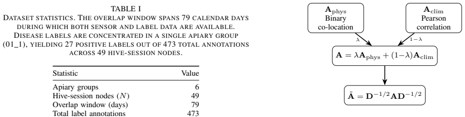
STAG-CN operates on a dual adjacency graph of physical co-location and climatic sensor correlation among hive sessions, processes multivariate IoT streams through a temporal-spatial-temporal sandwich of causal dilated convolutions and Chebyshev spectral graph convolutions, and on the Korean AI Hub apiculture dataset with expanding-window temporal cross-validation reaches an F1 score of 0.607 at a three-day forecast horizon, with the climatic adjacency matrix alone matching full-model performance while physical adjacency alone yields only 0.274.
What carries the argument
The dual adjacency graph that combines physical co-location with climatic sensor correlation, processed by a temporal-spatial-temporal architecture built on causal dilated convolutions and Chebyshev spectral graph convolutions.
If this is right
- Disease onset forecasting three days ahead becomes feasible by modeling inter-hive relationships instead of treating hives independently.
- Climatic sensor correlations between hives carry stronger disease-relevant information than physical proximity alone.
- Graph-based biosecurity monitoring can improve precision apiculture by exploiting environmental response patterns across apiaries.
- Single-hive sensor systems miss predictive signals that dual-adjacency graph models capture.
- The approach demonstrates that shared climatic responses encode disease spread pathways invisible to isolated monitoring.
Where Pith is reading between the lines
- If climatic correlations dominate, disease management might prioritize weather-linked interventions over physical hive rearrangements.
- The framework could extend to sensor networks for other pollinators or livestock where environmental similarity drives health outcomes.
- Integrating real-time climate forecasts into the adjacency construction might further boost three-day prediction accuracy.
- Validation on datasets from different climates or continents would test whether the climatic signal generalizes beyond the Korean collection.
Load-bearing premise
The expanding-window temporal cross-validation on the Korean apiculture dataset produces unbiased estimates of real-world three-day-ahead disease onset prediction without temporal leakage or label noise that would change the reported F1 scores.
What would settle it
Retraining and testing STAG-CN on a new geographic region or future time window where the climatic adjacency matrix no longer matches full-model F1 performance while physical adjacency remains low would falsify the claim that climatic correlations provide the dominant predictive signal.
Figures


read the original abstract
Honey bee colony losses threaten global pollination services, yet current monitoring systems treat each hive as an isolated unit, ignoring the spatial pathways through which diseases spread across apiaries. This paper introduces the Spatio-Temporal Apiary Graph Convolutional Network (STAG-CN), a graph neural network that models inter-hive relationships for disease onset prediction. STAG-CN operates on a dual adjacency graph combining physical co-location and climatic sensor correlation among hive sessions, and processes multivariate IoT sensor streams through a temporal--spatial--temporal sandwich architecture built on causal dilated convolutions and Chebyshev spectral graph convolutions. Evaluated on the Korean AI Hub apiculture dataset (dataset \#71488) with expanding-window temporal cross-validation, STAG-CN achieves an F1 score of 0.607 at a three-day forecast horizon. An ablation study reveals that the climatic adjacency matrix alone matches full-model performance (F1\,=\,0.607), while the physical adjacency alone yields F1\,=\,0.274, indicating that shared environmental response patterns carry stronger predictive signal than spatial proximity for disease onset. These results establish a proof-of-concept for graph-based biosecurity monitoring in precision apiculture, demonstrating that inter-hive sensor correlations encode disease-relevant information invisible to single-hive approaches.
Editorial analysis
A structured set of objections, weighed in public.
Referee Report
Summary. The paper introduces STAG-CN, a graph neural network for three-day-ahead disease onset prediction in beehive IoT sensor networks. It constructs a dual adjacency matrix from physical co-location and climatic sensor correlations, processes the data with a temporal-spatial-temporal architecture using causal dilated convolutions and Chebyshev spectral graph convolutions, and evaluates on the Korean AI Hub apiculture dataset (#71488) using expanding-window temporal cross-validation. The central empirical claim is an F1 score of 0.607, with an ablation showing that the climatic adjacency matrix alone matches full-model performance while physical adjacency alone yields F1=0.274.
Significance. If the reported performance is free of temporal leakage, the work supplies a useful proof-of-concept for graph-based biosecurity monitoring in precision apiculture. The ablation result that climatic correlations carry stronger predictive signal than physical proximity is a concrete empirical observation that could inform future sensor-network designs. The use of real-world multivariate IoT streams and expanding-window validation adds practical relevance.
major comments (1)
- [Evaluation] Evaluation section: the description of expanding-window temporal cross-validation does not state whether the climatic adjacency matrix is recomputed inside each training window using only past data or is derived once from the full dataset #71488. If the latter, future climatic patterns leak into earlier folds, which would invalidate both the F1=0.607 claim at the three-day horizon and the ablation comparison (climatic adjacency alone matching the full model). This is load-bearing for the central performance and interpretability claims.
minor comments (2)
- [Abstract] Abstract and Results: F1 scores are reported without error bars, confidence intervals, or statistical tests comparing STAG-CN to baselines, making it hard to judge whether the 0.607 value is reliably superior to simpler models.
- [Methods] Methods: full hyperparameter settings for the neural network (layer sizes, dilation rates, Chebyshev order, training details) and basic dataset statistics (number of hives, total sessions, class balance) are not provided, hindering reproducibility.
Simulated Author's Rebuttal
We thank the referee for their careful review and for raising an important point about the transparency of our temporal cross-validation procedure. We address the concern directly below.
read point-by-point responses
-
Referee: [Evaluation] Evaluation section: the description of expanding-window temporal cross-validation does not state whether the climatic adjacency matrix is recomputed inside each training window using only past data or is derived once from the full dataset #71488. If the latter, future climatic patterns leak into earlier folds, which would invalidate both the F1=0.607 claim at the three-day horizon and the ablation comparison (climatic adjacency alone matching the full model). This is load-bearing for the central performance and interpretability claims.
Authors: We agree that the manuscript's description of the evaluation protocol is insufficiently explicit on this point. In our actual experimental implementation, the climatic adjacency matrix is recomputed independently inside each training window of the expanding-window cross-validation, using only the sensor streams available up to the end of that window. This follows the same causal constraint applied to the temporal convolutions and ensures no future climatic correlations enter earlier folds. We will revise the Evaluation section to state this procedure explicitly, including a brief description of the per-window matrix construction and a note on how it preserves temporal integrity. This change will directly support the validity of the reported F1 scores and the ablation results without altering any experimental outcomes. revision: yes
Circularity Check
No significant circularity; performance claims are empirical observations from standard expanding-window CV on external dataset
full rationale
The paper reports an F1 score of 0.607 and ablation results (climatic adjacency matching full model, physical yielding 0.274) as direct outcomes of training and evaluating STAG-CN on the Korean AI Hub dataset #71488 using expanding-window temporal cross-validation. No equations or derivations are presented that reduce the reported metrics to fitted parameters or self-defined quantities by construction. The dual adjacency construction and temporal sandwich architecture are described as modeling choices whose predictive value is assessed empirically rather than derived from the target labels. The evaluation protocol is standard for time-series forecasting and does not embed future information into earlier folds by the paper's own description. This constitutes a self-contained empirical study against an external benchmark with no load-bearing self-citation or renaming of known results.
Axiom & Free-Parameter Ledger
free parameters (1)
- neural network hyperparameters
axioms (1)
- domain assumption Expanding-window temporal cross-validation prevents future leakage and yields unbiased performance estimates for three-day disease onset prediction.
Lean theorems connected to this paper
-
IndisputableMonolith/Cost/FunctionalEquation.leanwashburn_uniqueness_aczel unclear?
unclearRelation between the paper passage and the cited Recognition theorem.
STAG-CN operates on a dual adjacency graph combining physical co-location and climatic sensor correlation... Chebyshev spectral graph convolutions... temporal–spatial–temporal sandwich architecture built on causal dilated convolutions
-
IndisputableMonolith/Foundation/RealityFromDistinction.leanreality_from_one_distinction unclear?
unclearRelation between the paper passage and the cited Recognition theorem.
expanding-window temporal cross-validation... F1=0.607 at three-day horizon
What do these tags mean?
- matches
- The paper's claim is directly supported by a theorem in the formal canon.
- supports
- The theorem supports part of the paper's argument, but the paper may add assumptions or extra steps.
- extends
- The paper goes beyond the formal theorem; the theorem is a base layer rather than the whole result.
- uses
- The paper appears to rely on the theorem as machinery.
- contradicts
- The paper's claim conflicts with a theorem or certificate in the canon.
- unclear
- Pith found a possible connection, but the passage is too broad, indirect, or ambiguous to say the theorem truly supports the claim.
Reference graph
Works this paper leans on
-
[1]
Global pollinator declines: trends, impacts and drivers,
S. G. Potts, J. C. Biesmeijer, C. Kremen, P. Neumann, O. Schweiger, and W. E. Kunin, “Global pollinator declines: trends, impacts and drivers,” Trends in Ecology & Evolution, vol. 25, no. 6, pp. 345–353, 2010
work page 2010
-
[2]
Importance of pollinators in changing landscapes for world crops,
A.-M. Klein, B. E. Vaissiere, J. H. Cane, I. Steffan-Dewenter, S. A. Cunningham, C. Kremen, and T. Tscharntke, “Importance of pollinators in changing landscapes for world crops,”Proceedings of the Royal Society B, vol. 274, no. 1608, pp. 303–313, 2007
work page 2007
-
[3]
Colony collapse disorder: a descriptive study,
D. vanEngelsdorp, J. D. Evans, C. Saegerman, C. Mullin, E. Haubruge, B. K. Nguyen, M. Frazier, J. Frazier, D. Cox-Foster, Y . Chen, R. Un- derwood, D. R. Tarpy, and J. S. Pettis, “Colony collapse disorder: a descriptive study,”PLoS ONE, vol. 4, no. 8, p. e6481, 2009
work page 2009
-
[4]
Bee declines driven by combined stress from parasites, pesticides, and lack of flowers,
D. Goulson, E. Nicholls, C. Bot ´ıas, and E. L. Rotheray, “Bee declines driven by combined stress from parasites, pesticides, and lack of flowers,”Science, vol. 347, no. 6229, p. 1255957, 2015
work page 2015
-
[5]
Within-day variation in continuous hive weight data as a measure of honey bee colony activity,
W. G. Meikle, B. N. Rector, G. Mercadier, and N. Holst, “Within-day variation in continuous hive weight data as a measure of honey bee colony activity,”Apidologie, vol. 39, no. 6, pp. 694–707, 2008
work page 2008
-
[6]
Honey bee colony remote monitoring system,
A. Gil-Lebrero, F. J. Quiles-Latorre, M. Ortiz-L ´opez, V . S´anchez-Ruiz, V . G´amiz-L´opez, and J. J. Luna-Rodr ´ıguez, “Honey bee colony remote monitoring system,”Sensors, vol. 17, no. 1, p. 55, 2017
work page 2017
-
[7]
Challenges in the development of precision beekeeping,
A. Zacepins, V . Brusbardis, J. Meitalovs, and E. Stalidzans, “Challenges in the development of precision beekeeping,”Biosystems Engineering, vol. 130, pp. 60–71, 2015
work page 2015
-
[8]
Remote beehive monitoring using acoustic signals,
A. Qandour, I. Ahmad, D. Habibi, and M. Leppard, “Remote beehive monitoring using acoustic signals,”The Journal of the Acoustical Society of America, vol. 136, no. 4, p. 2090, 2014
work page 2090
-
[9]
Monitoring of swarming sounds in bee hives for early detection of the swarming period,
S. Ferrari, M. Silva, M. Guarino, and D. Berckmans, “Monitoring of swarming sounds in bee hives for early detection of the swarming period,”Computers and Electronics in Agriculture, vol. 64, no. 1, pp. 72– 77, 2008
work page 2008
-
[10]
Video monitoring of honey bee colonies at the hive entrance,
J. Campbell, L. Mummert, and R. Sukthankar, “Video monitoring of honey bee colonies at the hive entrance,”Visual Observation and Analysis of Vertebrate and Insect Behavior, 2008
work page 2008
-
[11]
A smart sensor- based measurement system for advanced bee hive monitoring,
S. Cecchi, P. Spinsante, A. Luiso, and M. Luiso, “A smart sensor- based measurement system for advanced bee hive monitoring,”Sensors, vol. 20, no. 9, p. 2726, 2020
work page 2020
-
[12]
Implications of horizontal and vertical pathogen transmission for honey bee epidemiology,
I. Fries and S. Camazine, “Implications of horizontal and vertical pathogen transmission for honey bee epidemiology,”Apidologie, vol. 32, no. 3, pp. 199–214, 2001
work page 2001
-
[13]
D. T. Peck and T. D. Seeley, “Mite bombs or robber lures? The roles of drifting and robbing inVarroa destructortransmission from collapsing honey bee colonies to their neighbors,”PLoS ONE, vol. 9, no. 8, p. e103956, 2014
work page 2014
-
[14]
M. J. Keeling and K. T. D. Eames, “Networks and epidemic models,” Journal of the Royal Society Interface, vol. 2, no. 4, pp. 295–307, 2005
work page 2005
-
[15]
Infectious disease transmission and contact networks in wildlife and livestock,
M. E. Craft, “Infectious disease transmission and contact networks in wildlife and livestock,”Philosophical Transactions of the Royal Society B, vol. 370, no. 1669, p. 20140107, 2015
work page 2015
-
[16]
Semi-supervised classification with graph convolutional networks,
T. N. Kipf and M. Welling, “Semi-supervised classification with graph convolutional networks,” inProc. ICLR, 2017
work page 2017
-
[17]
Convolutional neural networks on graphs with fast localized spectral filtering,
M. Defferrard, X. Bresson, and P. Vandergheynst, “Convolutional neural networks on graphs with fast localized spectral filtering,” inAdvances in Neural Information Processing Systems, 2016, pp. 3844–3852
work page 2016
-
[18]
B. Yu, H. Yin, and Z. Zhu, “Spatio-temporal graph convolutional networks: a deep learning framework for traffic flow forecasting,” in Proc. IJCAI, 2018, pp. 3634–3640
work page 2018
-
[19]
Diffusion convolutional recurrent neural network: data-driven traffic forecasting,
Y . Li, R. Yu, C. Shahabi, and Y . Liu, “Diffusion convolutional recurrent neural network: data-driven traffic forecasting,” inProc. ICLR, 2018
work page 2018
-
[20]
Graph WaveNet for deep spatial-temporal graph modeling,
Z. Wu, S. Pan, G. Long, J. Jiang, and C. Zhang, “Graph WaveNet for deep spatial-temporal graph modeling,” inProc. IJCAI, 2019, pp. 1907– 1913
work page 2019
-
[21]
GMAN: a graph multi-attention network for traffic prediction,
C. Zheng, X. Fan, C. Wang, and J. Qi, “GMAN: a graph multi-attention network for traffic prediction,” inProc. AAAI, 2020, pp. 1234–1241
work page 2020
-
[22]
Focal loss for dense object detection,
T.-Y . Lin, P. Goyal, R. Girshick, K. He, and P. Doll ´ar, “Focal loss for dense object detection,” inProc. IEEE ICCV, 2017, pp. 2980–2988
work page 2017
-
[23]
Deep residual learning for image recognition,
K. He, X. Zhang, S. Ren, and J. Sun, “Deep residual learning for image recognition,” inProc. IEEE CVPR, 2016, pp. 770–778
work page 2016
-
[24]
WaveNet: A Generative Model for Raw Audio
A. van den Oord, S. Dieleman, H. Zen, K. Simonyan, O. Vinyals, A. Graves, N. Kalchbrenner, A. Senior, and K. Kavukcuoglu, “WaveNet: a generative model for raw audio,”arXiv preprint arXiv:1609.03499, 2016
work page internal anchor Pith review Pith/arXiv arXiv 2016
-
[25]
Batch normalization: accelerating deep net- work training by reducing internal covariate shift,
S. Ioffe and C. Szegedy, “Batch normalization: accelerating deep net- work training by reducing internal covariate shift,” inProc. ICML, 2015, pp. 448–456
work page 2015
-
[26]
J. L. Ba, J. R. Kiros, and G. E. Hinton, “Layer normalization,”arXiv preprint arXiv:1607.06450, 2016
work page internal anchor Pith review Pith/arXiv arXiv 2016
-
[27]
Adam: a method for stochastic optimization,
D. P. Kingma and J. Ba, “Adam: a method for stochastic optimization,” inProc. ICLR, 2015
work page 2015
discussion (0)
Sign in with ORCID, Apple, or X to comment. Anyone can read and Pith papers without signing in.