REVIEW 4 major objections 5 minor 36 references
Implication of Kinetic Alfven Waves to Magnetic Field Turbulence Spectra: Earth's Magnetosheath
T0 review · 4 major / 5 minor · reviewed 2026-08-14 · deepseek-v4-flash
Pith's one-line read Kinetic Alfvén waves may explain steepened magnetosheath spectra
desk verdict The observational statistics on 337 magnetosheath intervals are a solid confirmation of known steepening, but the KAW simulation comparison is too loose to carry the theoretical claim. read the letter →
The pith
A machine-rendered reading of the paper's core claim, the machinery that carries it, and where it could break.
The reading
What carries the argument
The central object is the dimensionless two-fluid envelope equation for a kinetic Alfvén wave (Eq. (6)), in which nonlinearity enters through density fluctuations that adiabatically follow the wave amplitude and shift the wave frequency. The equation is evolved with a $128 \times 128$ de-aliased pseudo-spectral scheme from a slightly perturbed plane wave, and the resulting magnetic-field spectrum is compared with the observed one. On the data side, the machinery is the statistical slope-identification algorithm applied to Welch power spectra, together with minimum-variance analysis of the spectral matrix to obtain propagation angle $\theta_{kB}$ and compressibility $R$; Taylor's frozen-in hypothesis maps spacecraft frequencies to wavenumbers.
What would settle it
Determine the wavenumber spectrum of the same magnetosheath intervals directly from multi-point spacecraft measurements (Cluster tetrahedron or MMS) without invoking Taylor's hypothesis; if the break does not appear near $k\rho_i \simeq 0.05$ and the high-frequency slope does not fall between $-2.6$ and $-1.8$, the KAW explanation loses its observational basis. A direct measurement showing near-zero compressibility and parallel propagation for the high-frequency fluctuations would also contradict the KAW picture.
Extended reading notes
Core claim
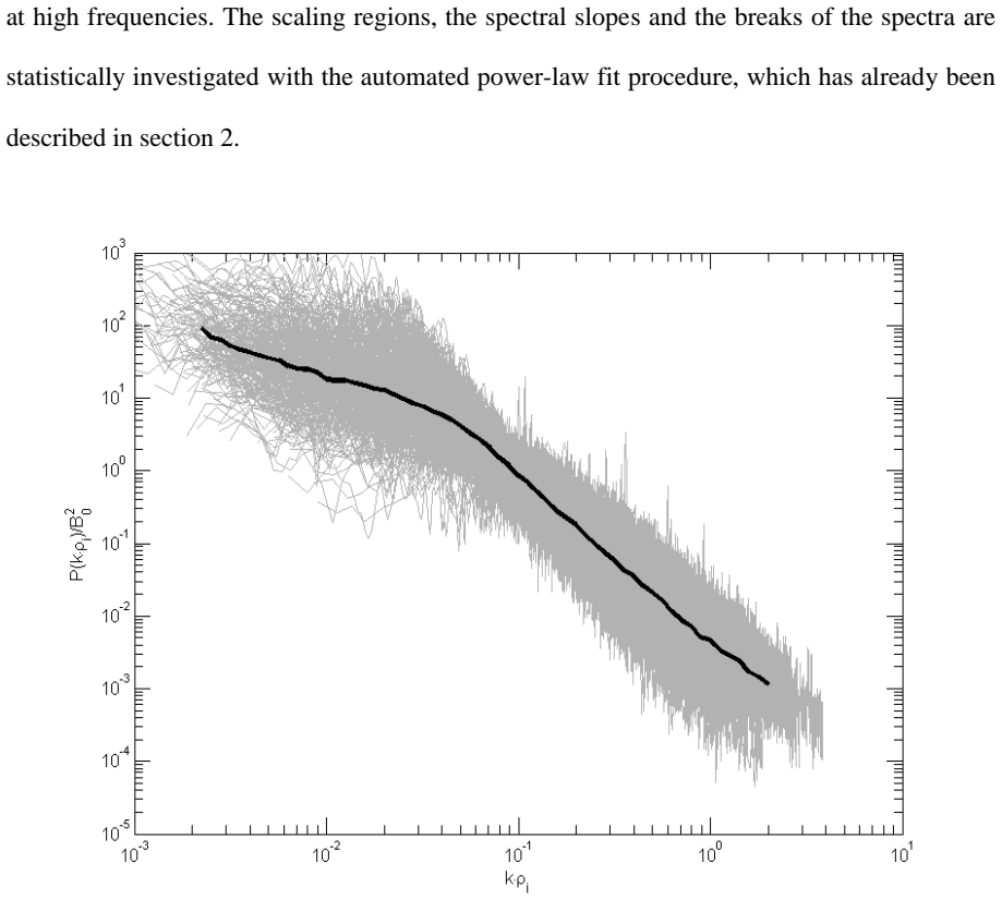
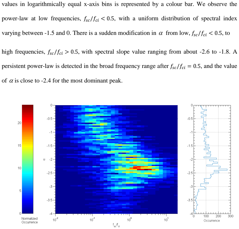
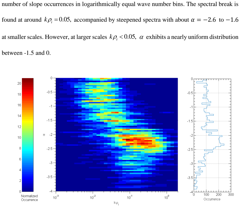
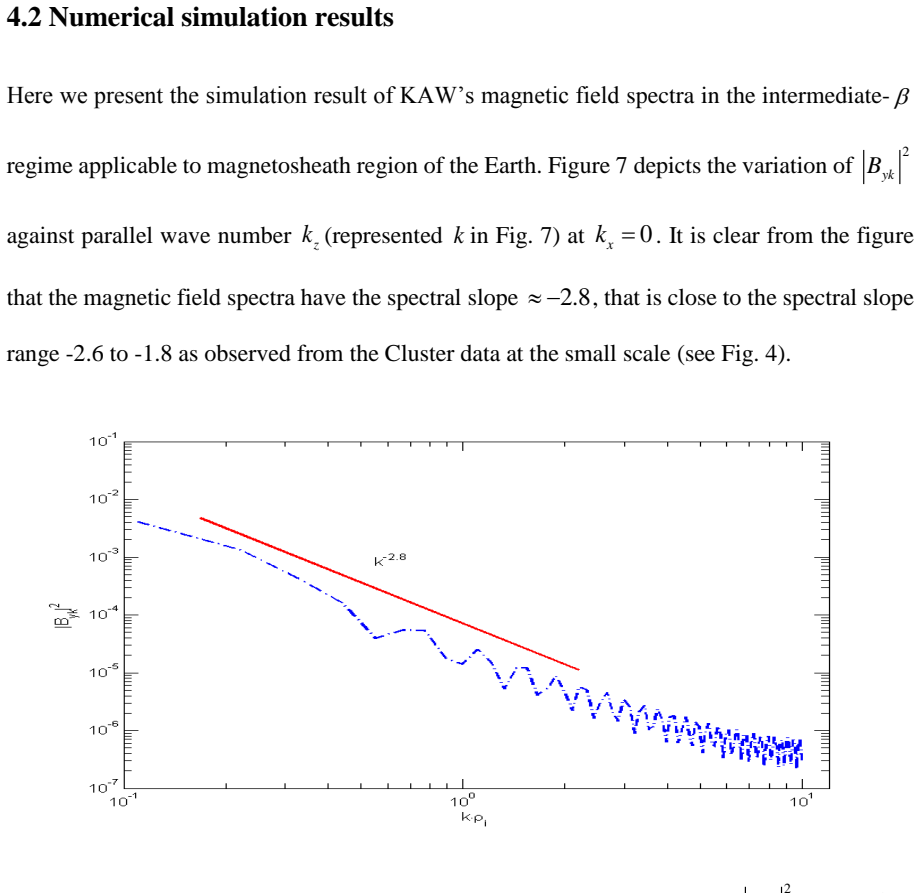
On its own terms, the paper establishes a statistical phenomenology and a candidate mechanism. The Cluster data show a clear transition: for $f_{sc}/f_{ci} < 0.5$ the spectral index $\alpha$ is broadly distributed between $-1.5$ and $0$, while for $f_{sc}/f_{ci} > 0.5$ the distribution peaks near $\alpha \approx -2.4$, with a persistent second power law between $-2.6$ and $-1.8$. In wavenumber units the break sits at $k\rho_i \simeq 0.05$. Propagation-angle and compressibility statistics indicate that low-frequency fluctuations are mostly perpendicular and mixed compressive/transverse, whereas above about $10 f_{ci}$ the angles spread over $30^\circ$-$90^\circ$ and the compressibility falls to $0.2 \lesssim R \lesssim 0.5$. The theoretical result is that the nonlinear evolution of kinetic Alfvén waves, simulated from a two-fluid envelope equation, produces a magnetic-field spectrum with slope near $-2.8$, close to the observed steep range. The paper therefore claims kinetic Alfvén waves are a plausible partial cause of the observed steepening, not that they are the only or definitively identified mechanism.
Load-bearing premise
The analysis assumes that each spacecraft-measured frequency can be converted to a spatial wavenumber by the bulk flow speed (Taylor's frozen-in hypothesis); if wave propagation speeds are not negligible, the reported spectral break and slopes in wavenumber space would change.
Editorial extensions
If this is right
- If kinetic Alfvén waves drive the steep range, the observed break near $k\rho_i \sim 0.05$ marks the scale at which KAW dynamics begins to dominate over larger-scale fluctuations.
- The near-absence of a Kolmogorov inertial range in most magnetosheath intervals would be a natural consequence of wave-dominated dynamics and finite shock-processing time, rather than a sign that no cascade exists.
- Magnetic spectra in other planetary magnetosheaths with similar plasma $\beta$ and temperature ratios should show the same break location and steep slopes if KAW turbulence is a general feature.
- The simulated slope near $-2.8$ gives a quantitative prediction that can be tested with higher-cadence or multi-spacecraft spectra without relying on Taylor's hypothesis.
Reading between the lines
- An extension implied by the paper is that the steepened range should carry KAW polarization signatures—magnetic fluctuations mostly perpendicular to $\mathbf{B}_0$ with a modest compressive component—which MMS data can check directly.
- The model's slope likely depends on $T_e/T_i$ and plasma $\beta$; sorting magnetosheath events by these parameters should reveal systematic shifts in the break scale and steepening rate.
- Because the simulation omits electron Landau damping, the observed steepening may combine KAW nonlinear transfer with kinetic dissipation; adding collisionless damping would predict whether the spectrum steepens further at electron scales.
- If KAW turbulence feeds the kinetic cascade, the energy should be deposited preferentially in electrons, so simultaneous electron temperature measurements could test the interpretation.
Signed reviews
Editorial analysis
A structured set of objections, weighed in public.
Referee Report
Summary. This paper analyzes 337 Cluster-1 magnetosheath intervals from 2007–2008, computes total magnetic field power spectra in spacecraft frequency and wavenumber domains, and uses a sliding-window fitting algorithm to extract spectral slopes, propagation angles from minimum variance analysis, and compressibility. The authors report low-frequency slopes between -1.5 and 0, a transition near 0.5 f_ci, steepened high-frequency slopes between -2.6 and -1.8 with a break at k rho_i ≈ 0.05, and broad propagation angles with moderate compressibility at high frequencies. They conjecture that kinetic Alfvén waves contribute to the small-scale steepening and support this with a two-fluid KAW model and a 2D pseudo-spectral simulation whose magnetic field spectrum has a slope near -2.8. The paper concludes that the simulated and observed spectra are analogous.
Significance. If the KAW interpretation were quantitatively established, the paper would provide a useful link between statistical magnetosheath observations and kinetic turbulence modeling, complementing earlier work by Zimbardo et al. and Tao et al. The observational statistical analysis covers a large event set and combines slope statistics with wave diagnostics, which is a strength; the data selection and spectral procedures are described in enough detail to be reproduced. The main limitation is that the quantitative comparison between simulation and observation is not yet convincing: the simulated spectrum is a different observable than the measured one and its slope is outside the quoted observed range. Thus the paper is better seen as presenting a plausible conjecture rather than a demonstrated implication.
major comments (4)
- [Section 4.2 (Fig. 7) versus Section 2.2 (Figs. 2 and 4)] The simulated spectrum plotted in Fig. 7 is |B_y(k_z)|^2 on the cut k_x=0 for a single transverse component, whereas the observed spectra in Figs. 2 and 4 are total-|B| spectra mapped along the spacecraft flow direction using the Taylor hypothesis. Because the flow direction is generally not parallel to the mean magnetic field, and because the observed high-frequency fluctuations have propagation angles broadly distributed between about 30 and 90 degrees (Fig. 5) with compressibility 0.2–0.5 (Fig. 6), the slope of a one-dimensional component cut along the parallel direction need not equal the slope of the observed trace spectrum. Please demonstrate that the simulated quantity is the same observable as the measured one, for example by computing an angle-averaged or flow-directed total-|B| spectrum from the model, or restrict the claim accordingly.
- [Section 4.2 and Section 5] The simulated spectral slope of about -2.8 lies outside the observed range -2.6 to -1.8 quoted in the abstract, Section 4.1, and Fig. 4, and it also differs from the most probable value of -2.4. Calling this 'close' is not quantitatively justified. Please provide a statistical comparison, such as the distribution of simulated slopes over an ensemble of realizations or a sensitivity study over the model parameters, and state explicitly whether the model reproduces the observed range or only a nearby value.
- [Section 5] The Taylor-hypothesis conditional analysis is described in the text but the results are not shown: the authors state that the basic statistical results remain unchanged for events with V_flow < 150 km/s (111 events) and V_flow > 219 km/s (112 events), but no figure or table is provided. Since the wavenumber-domain results and the break at k rho_i ≈ 0.05 (Fig. 4) rely directly on the Taylor mapping, please include the conditional results so that the reader can verify the claimed insensitivity to the flow speed.
- [Section 4.1 (Figs. 3 and 4)] The spectral slope distributions are reported without error bars or confidence intervals, and the scaling-range definition depends on an adjustable window length L and the sliding-fit procedure. Please quantify the uncertainty of the slope values (for example, with bootstrap resampling or interquartile ranges) to establish that the high-frequency range -2.6 to -1.8 and the break at k rho_i ≈ 0.05 are robust features rather than artifacts of the fitting algorithm.
minor comments (5)
- [Section 3.1 (Eq. 6)] The definitions of the dimensionless parameters Gamma_1 and Gamma_2 following Eq. (6) are unclear as printed, appearing to contain i and i^2 factors; please fix the notation and provide the intermediate algebra from Eq. (5) to Eq. (6) in an appendix or on request.
- [Abstract and Section 4.1] The expression '0.1 < R > 0.9' appears to be a typographical error for 0.1 ≤ R ≤ 0.9; please correct it.
- [Section 5] The sentence 'The conditional analyses prove that our results reliably characterise the spectral behaviour' is too strong given that the results are not shown; please soften the wording or include the analysis.
- [Throughout] The name 'Alfvèn' should be 'Alfvén', and the reference 'Kairmabadi' should be 'Karimabadi'; there are also several garbled mathematical expressions, for example '2.8k−' in Section 4.2, which should read '≈ -2.8'.
- [Section 2.2] The sentence 'the first three data pairs of the Welch spectra are skipped' is ambiguous; please clarify what is being skipped and why.
Circularity Check
No significant circularity; the simulated KAW spectrum is not fitted to the observed slopes, though self-cited model setup and quantity mismatches weaken the comparison.
full rationale
The paper's claimed derivation chain is: Cluster observations produce independent spectral-slope statistics; the authors conjecture KAWs as a possible cause; a two-fluid KAW equation (Eq. 6) with stated plasma parameters and initial condition (Eq. 7) is simulated; the simulated spectrum is then compared with the observed slopes. The simulation output is not obtained by fitting the observed spectral indices: the slope of about -2.8 in Fig. 7 emerges from the dynamical equation and the chosen initial perturbation, not from the observed -2.6 to -1.8 range. Thus there is no self-definitional or fitted-input-called-prediction circularity. The governing equation and initial condition are attributed partly to the authors' prior work (Dwivedi et al. 2012, 2013; Dwivedi & Sharma 2013), but these self-citations are not load-bearing in the circular sense: the equation is also traced to Shukla and Stenflo (1999, 2000), and the cited prior works do not assert the observational result. The comparison is weakened by legitimate scientific concerns -- the simulated quantity |B_y(k_z)|^2 at k_x=0 differs from the observed total-field spectrum along the flow, and -2.8 is outside the quoted observed range -- but these are correctness/evidence limitations, not circular reductions. The Taylor-hypothesis conditional analysis is described but not shown, which is an evidence gap rather than a construction of the result. Overall, the observational and theoretical parts remain independent, so the circularity score is low.
Assumptions & free parameters
free parameters (5)
- pump KAW frequency omega0 =
0.01 omega_ci
- pump perpendicular wavenumber k_x0 rho_i =
0.01
- initial perturbation amplitude and scale =
amplitude 0.1, kappa_x = kappa_z = 0.1
- spectral slope window L =
0.3 times the range of alpha(f)
- signal-to-noise truncation threshold =
2
assumptions (5)
- domain assumption Taylor's frozen-in flow hypothesis applies to all magnetosheath intervals.
- domain assumption The minimum variance eigenvector gives the wave propagation direction.
- domain assumption Two-fluid drift approximation with isothermal electrons and ions and adiabatic density response.
- domain assumption Weak nonlinearity and a plane-wave envelope ordering with d_x >> d_z.
- ad hoc to paper The pump KAW frequency and perpendicular wavenumber are small (0.01 omega_ci and 0.01 rho_i).
Cite this review
Pith. "Pith review of Implication of Kinetic Alfven Waves to Magnetic Field Turbulence Spectra: Earth's Magnetosheath." pith.science (2026). https://pith.science/paper/5XWGX7LS
@misc{pith2026190802533,
  author       = {Pith},
  title        = {Pith review of: Implication of Kinetic Alfven Waves to Magnetic Field Turbulence Spectra: Earth's Magnetosheath},
  year         = {2026},
  howpublished = {\url{https://pith.science/paper/5XWGX7LS}},
  note         = {Machine review of arXiv:1908.02533}
}
read the original abstract
In the present paper, we investigate the power-law behaviour of the magnetic field spectra in the Earths magnetosheath region using Cluster spacecraft data under solar minimum condition. The power spectral density of the magnetic field data and spectral slopes at various frequencies are analysed. Propagation angle and compressibility are used to test the nature of turbulent fluctuations. The magnetic field spectra have the spectral slopes between -1.5 to 0 down to spatial scales of 20 ion gyroradius and show clear evidence of a transition to steeper spectra for small scales with a second power-law, having slopes between -2.6 to -1.8. At low frequencies, f_sc<0.3f_ci(where f_ci is ion gyro-frequency), propagation angle approximately 90 degrees to the mean magnetic field, B_0, and compressibility shows a broad distribution, 0.1 < R > 0.9. On the other hand at f_sc>10f_ci, the propagation angle exhibits a broad range between 30-90 degree while 'R' has a small variation: 0.2 < R > 0.5. We conjecture that at high frequencies, the perpendicularly propagating Alfven waves could partly explain the statistical analysis of spectra. To support our prediction of kinetic Alfven wave-dominated spectral slope behaviour at high frequency, we also present a theoretical model and simulate the magnetic field turbulence spectra due to the nonlinear evolution of kinetic Alfven waves. The present study also shows the analogy between the observational and simulated spectra.
Figures

Figures from the paper (4 more)


Reference graph
Works this paper leans on
-
[1]
Balogh, A., Carr, C. M., Acuna, M. H., Dunlop, M. W., Beek, T. J., Brown, P. et al.: Annales Geophys. 19, 1207 (2001). Bavassano Cattaneo, M. B., Moreno, G., Russo, G., Richardson, J. D.: J. Geophys. Res. 105, 23141-23152 (2000)
work page 2001
-
[2]
Boldyrev, S., Horaites, K., Xia, Q., Perez, J. C.: Astrophys. J. 777, 41 (2013)
work page 2013
-
[3]
R., Sahraoui, F, Andriopoulou, M., Le Contel, O
Breuillard, H., Matteini, L., Argall, M. R., Sahraoui, F, Andriopoulou, M., Le Contel, O. et al.: Astrophys. J. 859, 127 (2018)
work page 2018
- [4]
-
[5]
Carr, C., Brown, P., Alconcel, L. -N. et al.: User guide to the FGM measurements in the Cluster Active Archive, (2014)
work page 2014
-
[6]
Chen, C.H.K., Leung, L., Boldyrev, S., Maruca, B.A., Ba le, S.D.: Geophys. Res. Lett. 28 , 41 (2014)
work page 2014
-
[7]
Chhiber, R., Chasapis, A., Bandyopadhyay, R., Parashar, T. N., Matthaeus, W. H., Maruca, B. A., Moore, T. E., Burch, J. L., Torbert, R. B., Russelll, C. T., Le Contel, O. et al: J. Geophys. Res.: Space Phys. 123, 12 (2018). Décréau, P. M. E., Fergeau, P., Krannosels’kikh, V. et al.: Space Sci. Rev. 79, 157– 193 (1997). 24 | P a g e
work page 2018
-
[8]
Dwivedi, N. K., Schmid, D., Narita, Y. et al.: Earth, Planets and Space 67, 137 (2015)
work page 2015
Show all 36 references
-
[9]
K., Sharma, R
Dwivedi, N. K., Sharma, R. P.: Phys. of Plasmas 20, 042308 (2013)
2013
-
[10]
K., Batra, K., Sharma, R
Dwivedi, N. K., Batra, K., Sharma, R. P.: J. Geophys. Res. 117, A07201 (2012)
2012
-
[11]
K., Sharma, R
Dwivedi, N. K., Sharma, R. P., Batra, K.: Astrophys. Space Sci. 343: 19-26 (2013)
2013
-
[12]
Franci, L., Landi, S., Matteini, L., Verdini, A., Hellinger, P.: Astrophys. J. 833, 91 (2016)
2016
-
[13]
Franci, L., Landi, S., Verdini, A., Matteini, L., Hellinger, P.: Astrophys. J. 853, 26 (2018)
2018
-
[14]
T., Thomsen, M
Gosling, J. T., Thomsen, M. F., Bame, S. J.: Geophys. Res. 94, 10011-10025 (1989)
1989
-
[15]
F., Jenko, F.: Phys
Groselj, D., Mallet, A., Loureiro, N. F., Jenko, F.: Phys. Rev. Lett. 120, 105101 (2018)
2018
-
[16]
K.: Astrophys
Dougherty, M. K.: Astrophys. J. Lett. 813, L29 (2015)
2015
-
[17]
Y., Sahraoui, F., Deng, X
Huang, S. Y., Sahraoui, F., Deng, X. H., He, J. S., Yuan, Z. G., Zhou, M., Pang, Y., Fu, H. S.: Astrophys. J. Lett. 836, L10 (2017)
2017
-
[18]
Y., Hadid, L
Huang, S. Y., Hadid, L. Z., Sahraoui, F., Yuan, Z. G., Deng, X. H.: Astrophys. J. Lett. 836, L10 (2017)
2017
-
[19]
et al.: Phys
Kairmabadi, H., Roytershteyn, V., Wan, M. et al.: Phys. of Plasmas 20, 012303 (2013)
2013
-
[20]
P., Singh, H
Kumar, S., Sharma, R. P., Singh, H. D.: Phys. of Plasmas 16, 072903 (2009)
2009
-
[21]
Kovacs, P., Facsko, G., Dandouras, I.: Planetary and Space Science 92, 24 (2014)
2014
-
[22]
J., Smith, C
Leamon, R. J., Smith, C. W., Ness, N. F. et al.: J. Geophys. Res. 104, 22331 (1999)
1999
-
[23]
Matteini, L., Alexandrova, O., Chen, C. H. K., Lacombe, C: MNRAS 466, 945-951 (2016)
2016
-
[24]
L., Russel, C
McPherron, R. L., Russel, C. T., Coleman, P. J.: Space Sci. Rev. 13, 411 (1972). Remé, H., Aoustin, C., Bosqued, J. M., Dandouras, I. et al.: Ann. Geophys. 19, 1303 (2001)
1972
-
[25]
P., Modi, K
Sharma, R. P., Modi, K. V.: Phys. of Plasmas 20, 08230 (2013)
2013
-
[26]
P., Malik, M.: Astron
Sharma, R. P., Malik, M.: Astron. Astrophys. 457, 675 (2006)
2006
-
[27]
P., Singh, H
Sharma, R. P., Singh, H. D.: J. Astrophys. Astr. 29, 239 (2008)
2008
-
[28]
K., Stenflo, L.: Phys
Shukla, P. K., Stenflo, L.: Phys. Plasmas 6, 4120–4122 (1999). 25 | P a g e
1999
-
[29]
K., Stenflo, L.: Phys
Shukla, P. K., Stenflo, L.: Phys. Plasmas 7, 2738–2739 (2000)
2000
-
[30]
de, Chust, T., Kasahara, S., Retinò, A.: J
Tao, C., Sahraoui, F., Fontaine, D., Patoul, J. de, Chust, T., Kasahara, S., Retinò, A.: J. Geophys. Res. 120, 2477-2493 (2015)
2015
-
[31]
I.: Proc
Taylor, G. I.: Proc. Roy. Soc. London A 164, 476 (1938)
1938
-
[32]
M., Slavin, J
Uritsky, V. M., Slavin, J. A., Khazanov, G. V., Donovan, E. F., Boardsen, S. A., Anderson, von Papen, M. V., Saur, J., Alexandrova, O.: J. Geophys. Res. 119, 2797 (2013). Vörös, Z., Zhang, T. L., Leubner, M. P. et al.: J. Geophys. Res. 113, E00B21 (2008)
2013
-
[33]
D.: IEEE Transactions on Audio and Electroacoustics 15, 7073 (1967)
Welch, P. D.: IEEE Transactions on Audio and Electroacoustics 15, 7073 (1967)
1967
-
[34]
V., Khodachenko, M
Zaqarashvili, T. V., Khodachenko, M. L., Rucker, H. O.: Astron. Astrophys. 529, A82 (2011)
2011
-
[35]
V., Khodachenko, M
Zaqarashvili, T. V., Khodachenko, M. L., Soler, R.: Astron. Astrophys. 549, A113 (2013)
2013
-
[36]
Zimbardo, G., Greco, A., Sorriso-Valvo, L., Perri, S., et al.: Space Sci. Rev. 156, 89 (2010)
2010
Reviewed August 14, 2026 · model on record in the stance chip above.
Discussion (0). Continue with ORCID to comment.