REVIEW 3 major objections 3 minor 33 references
Imaging with highly incomplete and corrupted data
T0 review · 3 major / 3 minor · reviewed 2026-08-14 · deepseek-v4-flash
Pith's one-line read A noise collector makes l1 imaging stable under noise
desk verdict The noise-collector idea is promising, but the random collector used in the experiments cannot satisfy the paper's own coherence conditions, and the proof of Lemma 3 has a gap, so the numerics and theory are not connected as claimed. read the letter →
The pith
A machine-rendered reading of the paper's core claim, the machinery that carries it, and where it could break.
The reading
What carries the argument
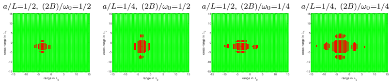
The load-bearing object is the noise collector matrix $C$, which is appended to the measurement matrix $A$ to form $D=[A|C]$. The construction in Proposition 2 iteratively adds unit-norm columns that are nearly orthogonal to all previous columns (inner products below $1/(3M)$); a volume-growth count shows termination after $\Sigma\lesssim e^N$ steps, and the representation built along the way gives $\gamma\le 18M^2$. The companion tool from Proposition 1 is the notion of a vicinity—the set of columns of $A$ almost parallel to a support column—whose non-overlap lets the error be decomposed into a coherent misfit inside vicinities and an incoherent 'grass' remainder, both controlled by $\gamma\delta$.
What would settle it
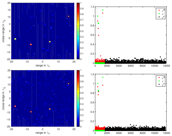
Take the paper's high-resolution setup (K = 3721, N = 625, SNR = 0 dB, random Gaussian noise collector with $\Sigma\approx 12000$) and increase $N$ to 1369 and 2500 while keeping the scene fixed; if the $\ell^1$ reconstruction error or the incoherent 'grass' grows with $N$ despite the noise collector, or if for any of these $N$ the random $C$ has $\max_{i,j}|\langle a_i,c_j\rangle|>1/(3M)$, the practical stabilization claim fails.
Extended reading notes
Core claim
The central claim is that plain $\ell^1$-minimization is unstable for high-resolution imaging with noisy data, because the minimal-$\ell^1$ solution obeys $\|\rho\|_1\le\gamma\|b\|_2$ with $\gamma=O(\sqrt{N})$, so the error bounds in Proposition 1 scale with $\sqrt{N}$ and worsen as more measurements are taken. The paper's remedy is the augmented system $[A|C]\rho=b$, where $C$ is a noise collector whose columns are incoherent with $A$ and with each other; Proposition 2 constructs such a $C$ with $\Sigma\lesssim e^N$ columns and proves the new constant satisfies $\gamma\le 18M^2$, independent of $N$. The proof is constructive: it builds $C$ column by column using a volume-growth argument, showing that every unit-norm data vector has a representation over the augmented columns with $\ell^1$ norm at most $18M^2$. The paper then demonstrates numerically, for additive uncorrelated Gaussian noise, that a random $C$ with $\Sigma\approx 10K$ columns behaves like the theoretical collector and yields clean images at SNR 0 dB.
Load-bearing premise
The practical claim depends on a random matrix with only about ten times as many columns as the image pixels behaving like the theoretical noise collector, which the proof requires to have exponentially many columns; the paper verifies only numerically that the necessary coherence conditions hold in this regime.
Editorial extensions
If this is right
- Plain l1 imaging degrades as the data dimension grows: for a fixed noise level $\delta$, the error bounds (15)–(16) grow like $\gamma\delta$ with $\gamma\propto\sqrt{N}$, so adding receivers or frequencies can hurt rather than help.
- With a noise collector satisfying the Proposition 2 conditions, the error constant becomes $\gamma\le 18M^2$, so the number of measurements no longer controls the noise sensitivity.
- The noise collector works by providing a frame on which the noise vector can be represented with small $\ell^1$ norm, separating the image content from the contaminating noise.
- For sparse noise (few corrupted entries), the identity matrix serves as the noise collector, linking this method to standard robust-principal-component-analysis style recovery.
Reading between the lines
- If the random-matrix regime is proven, the noise collector becomes a parameter-free add-on: the same random $C$ stabilizes l1 imaging across array sizes and frequencies, and the paper's numerics suggest $\Sigma\approx 10K$ is enough.
- A testable extension is to build $C$ adaptively from the observed residual rather than randomly, which could reduce $\Sigma$ for structured noise such as clutter or colored noise.
- The $\gamma\propto\sqrt{N}$ instability implies that in existing l1 imaging pipelines, increasing the aperture or bandwidth with noisy data can worsen the image; this counterintuitive prediction can be checked in the field.
- For non-Gaussian or correlated noise, the paper's framework prescribes a noise library tailored to the noise, but gives no theorem; experiments with colored noise would map the boundary of the practical claim.
Signed reviews
Editorial analysis
A structured set of objections, weighed in public.
Referee Report
Summary. The paper studies l1-minimization for sparse imaging from underdetermined linear systems Aρ=b with noisy data. It claims that for imaging matrices the stability constant γ in the error bound grows like sqrt(N), so l1-imaging degrades as the number of measurements grows, and it proposes augmenting A with a 'noise collector' matrix C so that the augmented system [A|C] has a stability constant γ≤18M^2 independent of N. Proposition 1 is intended to provide coherence-based stability estimates via 'vicinities' of the support columns, Proposition 2 constructs an exponential-size noise collector, and Section 4 reports numerical simulations with a random collector of moderate size (Σ≈10K).
Significance. If correct, the paper would give a useful explanation of a counterintuitive noise sensitivity of l1-imaging and a constructive remedy, with a parameter-free bound γ≤18M^2 for the augmented system. The idea of absorbing noise in an auxiliary dictionary is appealing and the numerical images support the possibility that something of the kind works. However, the central theoretical result is not merely under-proved: Proposition 1 is false as stated, and the numerical collector used in Section 4 does not satisfy the coherence assumptions of Proposition 2. As a result, the paper's main claims are not established.
major comments (3)
- [§3.1, Proposition 1 and Appendix A, Lemma 3] Proposition 1 is false as stated. Take N=2, K=4, M=2, ε=0.1, a1=(1,0)^T, a2=(0,1)^T, a3=(1,ε)^T/√(1+ε^2), a4=(ε,1)^T/√(1+ε^2), and ρ=(1,1,0,0) with b=a1+a2. The vicinities are S1={1,3} and S2={2,4}, which are disjoint, and Υ={1,2,3,4} contains no collinear vectors. Yet x=(0,0,u,u) with u=√(1+ε^2)/(1+ε)≈0.914 satisfies Ax=b and has l1-norm ≈1.828<2=||ρ||_1, so the minimal l1 solution is not ρ. This contradicts the δ=0 exact recovery statement of Proposition 1 and also contradicts inequality (30) in Lemma 3. The proof's displayed identity is vacuous because A(ρ−ξ)=0 makes both sides zero, and the subsequent inequality is not derived from the identity; the gap is not a presentation issue but reflects that the non-overlap condition with threshold 1/(3M) is insufficient.
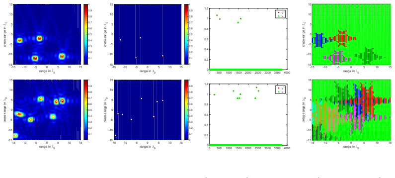
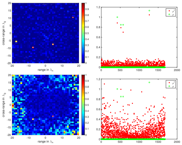
- [§4, Eqs. (18)–(19), Figures 4, 7, 8] The random noise collector used in the numerical experiments cannot satisfy the coherence conditions (18)–(19). For N=625 and Σ=12000 with i.i.d. Gaussian columns of variance 1/625, the inner product of two independent normalized columns has standard deviation 0.04, so the maximum over the roughly 7.2×10^7 column pairs is of order 0.24, far above the allowed thresholds 1/(3M)=0.083 for M=4 and 0.042 for M=8. The statement in Section 4 that conditions (18) and (19) are 'checked and satisfied' is therefore inconsistent with the statistics of the construction. Consequently, the numerical demonstrations in Figures 4, 7 and 8 are not connected to Proposition 2, and the practical claim is supported only by a few displayed images, without quantitative error metrics, multiple realizations, or code/data.
- [§3.1, Proposition 2] The termination step of Proposition 2 asserts that at the end of the iteration, condition (22) holds for every unit vector b, but the proof does not explicitly justify this assertion. If (22) failed for some b, then b could be added as a new column while preserving the incoherence bounds (18)–(19), so termination would not have occurred; this argument is implicit but should be stated. This gap is potentially fixable, unlike the counterexample to Proposition 1, but it is part of the proof of the central γ≤18M^2 bound and should be addressed in any revision.
minor comments (3)
- [§4] The noisy-data experiments report only images; no quantitative reconstruction errors, support errors, or signal-to-noise ratios of the reconstructions are given, and no indication of the number of random realizations is provided. Quantitative metrics and a reproducibility statement would be needed to assess the empirical claim.
- [§4] The columns of the random C are not exactly unit norm, while Proposition 2 requires ||d_j||=1; the authors mention that the norms tend to one as N→∞, but for finite N the O(1/√N) fluctuations should be accounted for when checking (18)–(19).
- [§3.1] The discussion of γ=O(√N) says 'let y be the minimum l2-norm solution of the problem Aρ=b such that its support has at most size N'; this is not the standard minimum l2-norm solution, and the wording should be clarified to say that one may choose a solution with at most N nonzero entries.
Circularity Check
No significant circularity: the theoretical framework is self-contained, and the numerical experiments illustrate rather than determine the bounds.
full rationale
The paper's derivation chain is not circular. Proposition 1 defines gamma in (13) as a quantity of the fixed matrix A (the supremum over data vectors c of the minimal l1 norm of a solution), and the error bounds (15)-(16) are then explicit consequences involving gamma times the noise level delta. This is a definition plus a proof, not a fitted parameter renamed as a prediction. Proposition 2 constructs the noise collector C by an iterative packing argument and derives gamma <= 18 M^2 from the resulting covering condition; the bound is proved, not assumed. The random C used in Section 4 is presented as a numerical ansatz: the paper states 'we check that conditions (18) and (19) are satisfied' and shows images as illustrations. Even if that check is numerically questionable at NS=625 and Sigma=12000, that is a gap between the theorem's sufficient conditions and the experiment, not a circular reduction, because the experiment supplies no constant used in the theorem. The only self-citations are the GeLMA solver [24] and prior scattering formulations [12,13]; these are implementation and extension references, and the main propositions do not depend on them. No equation is equivalent to an input by construction, and no fitted parameter is presented as a prediction. The practical gap identified by the skeptic concerns validity and numerical verification, not circularity.
Assumptions & free parameters
free parameters (3)
- Sigma (number of noise collector columns) =
12000 in experiments; abstract suggests ~10K
- Noise collector entry variance =
1/(NS)
- Vicinity threshold 1/(3M) =
1/(3M)
assumptions (4)
- domain assumption The imaging model is A rho = b with A known and columns normalized; rho is exactly M-sparse.
- domain assumption The vicinities S_j do not overlap for the true support T.
- domain assumption The data noise is additive, mean-zero, and uncorrelated.
- standard math Standard linear algebra facts: Gershgorin-type eigenvalue bounds and spherical packing estimates.
invented entities (1)
-
Noise collector matrix C and fictitious unknown components
Cite this review
Pith. "Pith review of Imaging with highly incomplete and corrupted data." pith.science (2026). https://pith.science/paper/5Z53FGST
@misc{pith2026190801479,
  author       = {Pith},
  title        = {Pith review of: Imaging with highly incomplete and corrupted data},
  year         = {2026},
  howpublished = {\url{https://pith.science/paper/5Z53FGST}},
  note         = {Machine review of arXiv:1908.01479}
}
abstract
We consider the problem of imaging sparse scenes from a few noisy data using an $l_1$-minimization approach. This problem can be cast as a linear system of the form $A \, \rho =b$, where $A$ is an $N\times K$ measurement matrix. We assume that the dimension of the unknown sparse vector $\rho \in {\mathbb{C}}^K$ is much larger than the dimension of the data vector $b \in {\mathbb{C}}^N$, i.e, $K \gg N$. We provide a theoretical framework that allows us to examine under what conditions the $\ell_1$-minimization problem admits a solution that is close to the exact one in the presence of noise. Our analysis shows that $l_1$-minimization is not robust for imaging with noisy data when high resolution is required. To improve the performance of $l_1$-minimization we propose to solve instead the augmented linear system $ [A \, | \, C] \rho =b$, where the $N \times \Sigma$ matrix $C$ is a noise collector. It is constructed so as its column vectors provide a frame on which the noise of the data, a vector of dimension $N$, can be well approximated. Theoretically, the dimension $\Sigma$ of the noise collector should be $e^N$ which would make its use not practical. However, our numerical results illustrate that robust results in the presence of noise can be obtained with a large enough number of columns $\Sigma \approx 10 K$.
Figures

Figures from the paper (5 more)



Reference graph
Works this paper leans on
-
[1]
F. Alizadeh, Interior point methods in semidefinite programming with applications to combinatorial optimization , SIAM J. Optim. 5 (1995), pp. 13–51
work page 1995
-
[2]
Beck, Amir , and Teboulle, Marc , A Fast Iterative Shrinkage- Thresholding Algorithm for Linear Inverse Problems , SIAM J. Img. Sci. 2 (2009), pp.183–202
work page 2009
-
[3]
L. Borcea and I. Kocyigit, Resolution analysis of imaging with 𝓁1 optimization, SIAM J. Imaging Sci. 8 (2015), pp. 3015–3050
work page 2015
-
[4]
L. Borcea and I. Kocyigit,A multiple measurement vector approach to synthetic aperture radar imaging, SIAM J. Imaging Sci. 11 (2018), pp. 770–801
work page 2018
-
[5]
L. Borcea and G. Papanicolaou and C. Tsogka, A resolution study for imaging and time reversal in random media , Contemporary Math. 333 (2003), pp. 63–77
work page 2003
-
[6]
Russell, Entropic regularization of the𝓁0 function, Springer Optim
Borwein, Jonathan M.and Luke, D. Russell, Entropic regularization of the𝓁0 function, Springer Optim. Appl. 49 (2011), Springer, pp. 65–92
work page 2011
-
[7]
Bruckstein, Alfred M. , Donoho, David L., Elad, Michael, From sparse solutions of systems of equations to sparse modeling of signals and images, SIAM Rev. 51 (2009), pp.34–81. 22
work page 2009
-
[8]
E.J Cand`es. J. K. Romberg, and T. Tao , Stable signal recovery from incomplete and inaccurate information, Communications on Pure and Applied Mathematics 59 (2006), pp. 1207–33
work page 2006
Show all 33 references
-
[9]
J Cand`es and T
E. J Cand`es and T. Tao, Near optimal signal recovery from random projections: universal encoding strategies?, IEEE Trans. Inf. Theory 52 (2006), pp. 5406–25
2006
-
[10]
E. J. Cand`es, Y. C. Eldar, T. Strohmer, and V. Voroninski , Phase Retrieval via Matrix Completion, SIAM J. Imaging Sci. 6 (2013), pp. 199–225
2013
-
[11]
E. J. Cand `es and C. Fernandez-Granda , Towards a mathemat- ical theory of super-resolution, Communications on Pure and Applied Mathematics 67 (2014), pp. 906-956
2014
-
[12]
A. Chai, M. Moscoso and G. Papanicolaou , Robust imaging of localized scatterers using the singular value decomposition and 𝓁1 opti- mization, Inverse Problems 29 (2013), 025016
2013
-
[13]
A. Chai, M. Moscoso and G. Papanicolaou, Imaging strong local- ized scatterers with sparsity promoting optimization , SIAM J. Imaging Sci. 10 (2014), pp. 1358–1387
2014
-
[14]
Chambolle and T
A. Chambolle and T. Pock, A first-order primal-dual algorithm for convex problems with applications to imaging, Journal of Mathematical Imaging and Vision 40 (2011), pp 120–145
2011
-
[15]
Donoho, Super-resolution via sparsity constraint, SIAM Journal on Mathematical Analysis 23 (1992), pp
D. Donoho, Super-resolution via sparsity constraint, SIAM Journal on Mathematical Analysis 23 (1992), pp. 1303–1331
1992
-
[16]
Donoho and M
D. Donoho and M. Elad, Optimally sparse representation in general (nonorthogonal) dictionaries via 𝓁1 minimization, Proceedings of the National Academy of Sciences 100 (2003), pp. 2197–2202
2003
-
[17]
Donoho, M
D. Donoho, M. Elad and V. Temlyakov, Stable recovery of sparse overcomplete representations in the presence of noise , IEEE Trans. In- formation Theory 52 (2006), pp. 6–18
2006
-
[18]
Efron, T
B. Efron, T. Hastie, I. Johnstone, and R. Tibshirani , Least angle regression, Annals of Statistics 32 (2004), pp. 407–499. 23
2004
-
[19]
Fannjiang and W
A. Fannjiang and W. Liao , Coherence pattern-guided compressive sensing with unresolved grids, SIAM J. Imaging Sci. 5 (2012), pp. 179– 202
2012
-
[20]
M. A. T. Figueiredo, R. D. Nowak, and S. J. Wright, Gradient projection for sparse reconstruction: application to compressed sensing and other inverse problems, IEEE Journal of Selected Topics in Signal Processing 1 (2007), pp.586–597
2007
-
[21]
I. F. Gorodnitsky, and B. D. Rao , Sparse Signal Reconstruction from Limited Data Using FOCUSS: A Re-weighted Minimum Norm Al- gorithm, Trans. Sig. Proc. 45 (1997), pp. 600–616
1997
-
[22]
Gribonval and M
R. Gribonval and M. Nielsen , Sparse representations in unions of bases, IEEE Transactions on Information Theory 49 (2003), pp. 3320– 3325
2003
-
[23]
J. N. Laska, M. A. Davenport and R. G. Baraniuk, Exact signal recovery from sparsely corrupted measurements through the Pursuit of Justice, 2009 Conference Record of the Forty-Third Asilomar Conference on Signals, Systems and Computers, Pacific Grove, CA, 2009, pp. 1556– 1560
2009
-
[24]
Moscoso, A
M. Moscoso, A. Novikov, G. Papanicolaou and L. Ryzhik , A differential equations approach to l1-minimization with applications to array imaging, Inverse Problems 28 (2012)
2012
-
[25]
Nedi´c, and D
A. Nedi´c, and D. P. Bertsekas, Incremental subgradient methods for non-differentiable optimization , SIAM J. Optim. 12 (2001), pp.109– 138
2001
-
[26]
Nesterov , A method of solving a convex programming problem with convergence rate O(1/k2), Soviet Mathematics Doklady 27 (1983), pp
Y. Nesterov , A method of solving a convex programming problem with convergence rate O(1/k2), Soviet Mathematics Doklady 27 (1983), pp. 372–376
1983
-
[27]
Nesterov , Gradient methods for minimizing composite objective function, Math
Y. Nesterov , Gradient methods for minimizing composite objective function, Math. Program., Ser. B 140 (2013), pp. 125–161
2013
-
[28]
M. R. Osborne, B. Presnell, and B.A. Turlach, A new approach to variable selection in least squares problems, IMA Journal of Numerical Analysis 20 (2000), pp. 389-403. 24
2000
-
[29]
Tibshirani, Regression shrinkage and selection via the Lasso , Jour- nal of the Royal Statistical Society, Series B 58 (1996), pp
R. Tibshirani, Regression shrinkage and selection via the Lasso , Jour- nal of the Royal Statistical Society, Series B 58 (1996), pp. 267–288
1996
-
[30]
Tropp , Just relax: Convex programming methods for identifying sparse signals in noise , IEEE Trans
J. Tropp , Just relax: Convex programming methods for identifying sparse signals in noise , IEEE Trans. Information Theory 52 (2006), pp. 1030–1051
2006
-
[31]
Tropp, A Gilbert, and M
J. Tropp, A Gilbert, and M. Strauss , Algorithms for simultane- ous sparse approximation. Part I: Greedy pursuit , Signal Processing 86 (2006), pp. 572–588
2006
-
[32]
Tropp, Algorithms for simultaneous sparse approximation
J. Tropp, Algorithms for simultaneous sparse approximation. Part II: Convex relaxation, Signal Processing 86 (2006), pp. 589–602
2006
-
[33]
M. H. Wright, The interior-point revolution in optimization: history, recent developments, and lasting consequences , Bull. Amer. Math. Soc. (N.S) 42 (2005), pp.39–56. A Proof of Proposition 1 We will now prove auxiliary lemmas that we will use in the proof of Propos- tion 1. ...
2005
Reviewed August 14, 2026 · model on record in the stance chip above.
Discussion (0). Continue with ORCID to comment.