Generating Input Distributions for Explaining Portfolio Optimization Pipelines
Pith reviewed 2026-06-25 20:19 UTC · model grok-4.3
The pith
Gradient-based sample generation interprets portfolio optimization pipelines by identifying macroeconomic conditions that produce specific outcomes.
A machine-rendered reading of the paper's core claim, the machinery that carries it, and where it could break.
Core claim
We propose a predict-optimize-explain framework that uses gradient-based sample generation to interpret various portfolio models by identifying macroeconomic conditions that induce specified portfolio outcomes. Unlike traditional feature-importance methods, this approach directly probes decision pipelines (predictive models coupled with portfolio optimization) by constructing economically meaningful what-if questions. We focus on four such questions: under what macroeconomic conditions a predict-then-optimize pipeline closes or reverses its return gap with a predict-and-optimize pipeline; what conditions lead a pipeline to diversify rather than concentrate its allocation; when a pipeline tra
What carries the argument
Gradient-based sample generation that produces input distributions to answer economically meaningful what-if questions about coupled prediction and optimization pipelines.
If this is right
- Macroeconomic conditions exist under which a predict-then-optimize pipeline closes or reverses its return gap relative to a predict-and-optimize pipeline.
- Certain input conditions cause a pipeline to shift from concentrated to diversified allocations.
- A pipeline trained only on calm markets can overtake one trained on crisis data under identifiable macroeconomic regimes.
- Conditions can be identified that allow any given pipeline to match a chosen benchmark return.
- The same generation technique can be applied to additional user-defined questions about portfolio objectives.
Where Pith is reading between the lines
- The technique could transfer to other domains that couple machine learning predictions with downstream optimization, such as supply chain or energy planning.
- Regulators might use the generated distributions to run targeted stress tests on reported portfolio strategies.
- The approach could be combined with real-time economic data feeds to produce ongoing explanations rather than one-time analyses.
Load-bearing premise
Gradient-based sample generation produces input distributions that remain economically meaningful and faithfully probe the pipelines without introducing artifacts from the generation process itself.
What would settle it
A test showing that the generated macroeconomic input distributions lead to portfolio outcomes that contradict observed historical market responses or economic intuition would falsify the claim that the samples validly probe the pipelines.
Figures
read the original abstract
We propose a predict-optimize-explain framework that uses gradient-based sample generation to interpret various portfolio models by identifying macroeconomic conditions that induce specified portfolio outcomes. Unlike traditional feature-importance methods, this approach directly probes decision pipelines (predictive models coupled with portfolio optimization) by constructing economically meaningful what-if questions. We focus on four such questions: under what macroeconomic conditions a predict-then-optimize pipeline closes or reverses its return gap with a predict-and-optimize pipeline; what conditions lead a pipeline to diversify rather than concentrate its allocation; when a pipeline trained on calm markets overtakes one trained through crises; and what conditions would let a pipeline match a benchmark return. These examples illustrate how our framework uncovers key behavioral differences between various decision pipelines. Beyond these cases, the proposed framework is flexible and can support a wide range of probing questions tailored to specific portfolio objectives. Our findings highlight the value of integrating prediction, optimization, and explanation to produce more robust and transparent portfolio strategies.
Editorial analysis
A structured set of objections, weighed in public.
Referee Report
Summary. The paper proposes a predict-optimize-explain framework that employs gradient-based sample generation to construct input distributions answering four specific what-if questions about portfolio optimization pipelines. These questions target conditions under which a predict-then-optimize pipeline closes its return gap with a predict-and-optimize pipeline, when a pipeline diversifies rather than concentrates allocations, when a calm-market-trained pipeline overtakes a crisis-trained one, and when a pipeline matches a benchmark return. The approach is illustrated through explicit derivations of the corresponding distributions and resulting allocation shifts, with the framework presented as flexible for additional probing questions.
Significance. If the generated distributions remain faithful to the underlying models without introducing generation artifacts, the framework offers a targeted interpretability tool for coupled prediction-optimization systems that goes beyond feature-importance methods by directly probing decision outcomes. The explicit construction of the four examples from the models themselves, without additional unverifiable steps, strengthens the contribution as an illustrative methodology in operations research.
minor comments (3)
- The description of the gradient-based sample generation procedure would benefit from an explicit algorithm box or pseudocode to make the method reproducible from the text alone.
- A summary table listing the four probing questions, the derived input distributions, and the observed allocation shifts would improve clarity and allow readers to compare the behavioral differences at a glance.
- Notation for the generated input distributions (e.g., symbols for the macroeconomic variables and the optimization outputs) should be introduced once and used consistently across all examples.
Simulated Author's Rebuttal
We thank the referee for their positive summary of our work, recognition of its significance as an interpretability tool for predict-optimize pipelines, and recommendation of minor revision. The referee's description accurately reflects the manuscript's focus on gradient-based sample generation for four specific what-if questions in portfolio optimization.
Circularity Check
No significant circularity; framework is self-contained methodology
full rationale
The manuscript presents a predict-optimize-explain framework that constructs input distributions via gradient-based generation to probe portfolio pipelines. All load-bearing elements (four explicit probing questions, derived distributions, and allocation-shift illustrations) are generated directly from the coupled models by explicit construction rather than by fitting parameters to the target outputs or by self-citation chains. No equations or claims reduce to their own inputs by definition, and the work is framed as an illustrative methodology without invoking uniqueness theorems or ansatzes from prior self-work. The derivation chain therefore remains independent of the results it produces.
Axiom & Free-Parameter Ledger
Reference graph
Works this paper leans on
-
[1]
S. Agal, K. Raulji, and N. Odedra. A machine learning approach to risk based asset allocation in portfolio optimization.Scientific Reports, page 42263, 2025
2025
-
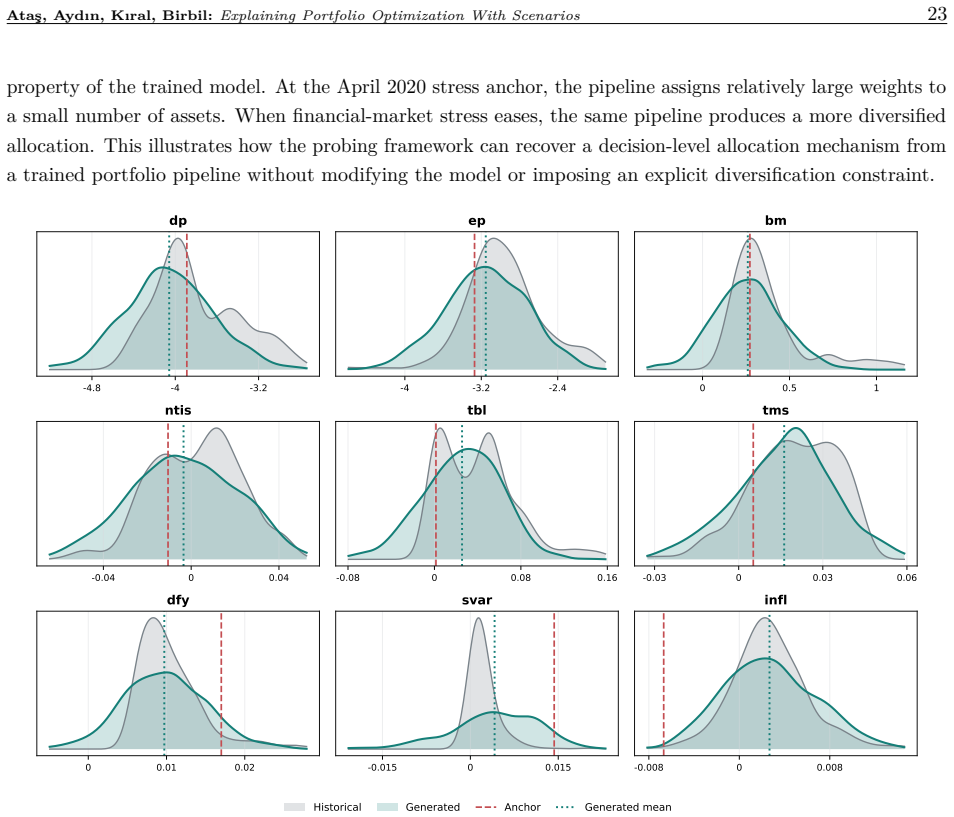
[2]
Agrawal, B
A. Agrawal, B. Amos, S. Barratt, S. Boyd, S. Diamond, and J. Z. Kolter. Differentiable convex optimization layers. InAdvances in Neural Information Processing Systems, volume 32, pages 9562–9574, 2019
2019
-
[3]
Anari, S
N. Anari, S. Chewi, and T.-D. Vuong. Fast parallel sampling under isoperimetry. InThe Thirty Seventh Annual Conference on Learning Theory, pages 161–185. PMLR, 2024
2024
-
[4]
H. T. Anis and R. H. Kwon. End-to-end, decision-based, cardinality-constrained portfolio optimization. European Journal of Operational Research, 320(3):739–753, 2025. doi: 10.1016/j.ejor.2024.08.030
-
[5]
Avramov, S
D. Avramov, S. Cheng, and L. Metzker. Machine learning versus economic restrictions: Evidence from stock return predictability.Management Science, 69(5):2587–2611, 2023
2023
-
[6]
O. Bastani, C. Kim, and H. Bastani. Interpreting blackbox models via model extraction.arXiv preprint arXiv:1705.08504, 2017
Pith/arXiv arXiv 2017
-
[7]
D. Bertsimas, V. Gupta, and N. Kallus. Data-driven robust optimization.Mathematical Programming, 167(2):235–292, 2018. doi: 10.1007/s10107-017-1125-8
-
[8]
Blanchet, L
J. Blanchet, L. Chen, and X. Y. Zhou. Distributionally robust mean-variance portfolio selection with wasserstein distances.Management Science, 68(9):6382–6410, 2022
2022
-
[9]
S. Boyd, K. Johansson, R. Kahn, P. Schiele, and T. Schmelzer. Markowitz portfolio construction at seventy.arXiv preprint arXiv:2401.05080, 2024
arXiv 2024
-
[10]
Butler and R
A. Butler and R. H. Kwon. Integrating prediction in mean-variance portfolio optimization.Quantitative Finance, 23(3):429–452, 2023
2023
-
[11]
A. Y. Chen and T. Zimmermann. Open source cross-sectional asset pricing.Critical Finance Review, 27 (2):207–264, 2022
2022
-
[12]
L. Chen, M. Pelger, and J. Zhu. Deep learning in asset pricing.Management Science, 70(2):714–750, 2024
2024
-
[13]
L. W. Cong, K. Tang, J. Wang, and Y. Zhang. AlphaPortfolio: Direct construction through deep reinforcement learning and interpretable AI.Social Science Research Network, 2020. SSRN working paper 3554486. Forthcoming in Management Science
2020
-
[14]
Costa and G
G. Costa and G. N. Iyengar. Distributionally robust end-to-end portfolio construction.Quantitative Finance, 23(10):1465–1482, 2023
2023
-
[15]
Diamond and S
S. Diamond and S. Boyd. CVXPY: A Python-embedded modeling language for convex optimization. Journal of Machine Learning Research, 17(83):1–5, 2016
2016
-
[16]
P. L. Donti, B. Amos, and J. Z. Kolter. Task-based end-to-end model learning in stochastic optimization. InProceedings of the 31st International Conference on Neural Information Processing Systems, NIPS’17, page 5490–5500, Red Hook, NY, USA, 2017. Curran Associates Inc. arXiv:1703.04529
Pith/arXiv arXiv 2017
-
[17]
A. Durmus and É. Moulines. On the geometric convergence for MALA under verifiable conditions.arXiv preprint arXiv:2201.01951, 2022
arXiv 2022
-
[18]
A. N. Elmachtoub and P. Grigas. Smart “predict, then optimize”.Management Science, 68(1):9–26, 2022. doi: 10.1287/mnsc.2020.3922. Ataş, Aydın, Kıral, Birbil:Explaining Portfolio Optimization With Scenarios33
-
[19]
A. N. Elmachtoub, J. C. N. Liang, and R. McNellis. Decision trees for decision-making under the predict-then-optimize framework. InProceedings of the 37th International Conference on Machine Learning, ICML’20. JMLR.org, 2020
2020
-
[20]
Estrella and F
A. Estrella and F. S. Mishkin. The yield curve as a predictor of U.S. recessions.Current Issues in Economics and Finance (FRBNY), 2(7), 1996
1996
-
[21]
J. P. M. Franco and M. P. Laurini. Integrating choquet portfolios and machine learning interpretability for robust cryptocurrency investment strategies.The Journal of Finance and Data Science, 11:100172, 2025
2025
-
[22]
Gilchrist and E
S. Gilchrist and E. Zakrajsek. Credit spreads and business cycle fluctuations.American Economic Review, 102(4):1692–1720, 2012
2012
-
[23]
Goyal and I
A. Goyal and I. Welch. A comprehensive look at the empirical performance of equity premium prediction. Review of Financial Studies, 21(4):1455–1508, 2008
2008
-
[24]
Goyal and I
A. Goyal and I. Welch. Predictordata2024.xlsx: Updated equity premium predictor data. Data file, 2024. Downloaded from https://www.hec.unil.ch/agoyal/
2024
-
[25]
S. Gu, B. Kelly, and D. Xiu. Empirical asset pricing via machine learning.The Review of Financial Studies, 33(5):2223–2273, 2020. doi: 10.1093/rfs/hhaa009
-
[26]
Hastings
W. Hastings. Monte Carlo sampling methods using Markov chains and their applications.Biometrika, 57:97–109, 1970
1970
-
[27]
Ho-Nguyen and F
N. Ho-Nguyen and F. Kılınç-Karzan. Risk guarantees for end-to-end prediction and optimization processes. Management Science, 68(12):8680–8698, 2022
2022
- [28]
-
[29]
Israel, B
R. Israel, B. Kelly, and T. J. Moskowitz. Can machines “learn” finance?Journal of Investment Management, 18(2):23–36, 2020
2020
-
[30]
J. Kim, S. Choi, Y. Lee, Y. Kim, Y. Choi, and Y. Lee. Decision by supervised learning with deep ensembles: A practical framework for robust portfolio optimization. InProceedings of the 34th ACM International Conference on Information and Knowledge Management, New York, NY, USA, 2025. ACM
2025
-
[31]
D. Kisiel and D. Gorse. Portfolio transformer for attention-based asset allocation. InArtificial Intelligence and Soft Computing, volume 13341 ofLecture Notes in Artificial Intelligence, pages 61–71. Springer, 2022. Also available as arXiv:2206.03246
arXiv 2022
-
[32]
C. Lau. A simple normal inverse gaussian-type approach to intraday value-at-risk estimation.Journal of Risk, 18(1), 2015
2015
-
[33]
Ledoit and M
O. Ledoit and M. Wolf. A well-conditioned estimator for large-dimensional covariance matrices.Journal of Multivariate Analysis, 88(2):365–411, 2004
2004
-
[34]
J. Lee, H. Jeon, H. Bae, and Y. Lee.Return Prediction for Mean-Variance Portfolio Selection: How Decision-Focused Learning Shapes Forecasting Models, page 114–122. Association for Computing Machin- ery, New York, NY, USA, 2025
2025
-
[35]
Mandi, J
J. Mandi, J. Kotary, S. Berden, M. Mulamba, V. Bucarey, T. Guns, and F. Fioretto. Decision-focused learning: Foundations, state of the art, benchmark and future opportunities.Journal of Artificial Intelligence Research, 80, Sept. 2024. Ataş, Aydın, Kıral, Birbil:Explaining Portfolio Optimization With Scenarios34
2024
-
[36]
Markowitz
H. Markowitz. Portfolio selection.The Journal of Finance, 7(1):77–91, 1952
1952
-
[37]
S. P. Meyn and R. L. Tweedie.Markov Chains and Stochastic Stability. Springer Science & Business Media, 2012
2012
-
[38]
R. M. Neal et al. MCMC using Hamiltonian dynamics.Handbook of Markov Chain Monte Carlo, 2(11): 2, 2011
2011
-
[39]
G. O. Roberts and J. S. Rosenthal. General state space Markov chains and MCMC algorithms.Probability Surveys, 1:20–71, 2004
2004
-
[40]
G. O. Roberts and R. L. Tweedie. Exponential convergence of Langevin distributions and their discrete approximations.Bernoulli, 2(4):341–363, 1996
1996
-
[41]
A. S. Uysal, X. Li, and J. M. Mulvey. End-to-end risk budgeting portfolio optimization with neural networks.Annals of Operations Research, 339:397–426, 2024
2024
-
[42]
P. Z. Wang, J. Liang, S. Chen, F. Fioretto, and S. Zhu. Gen-dfl: Decision-focused generative learning for robust decision making.arXiv preprint arXiv:2502.05468, 2025. doi: 10.48550/arXiv.2502.05468
-
[43]
C. Yin, R. Perchet, and F. Soupé. A practical guide to robust portfolio optimization.Quantitative Finance, 21(6):911–928, 2021
2021
-
[44]
C. Zhang, Z. Zhang, M. Cucuringu, and S. Zohren. A universal end-to-end approach to portfolio optimization via deep learning.arXiv preprint arXiv:2111.09170, 2021. Ataş, Aydın, Kıral, Birbil:Explaining Portfolio Optimization With Scenarios35 Appendix A. Macroeconomic Predictors.We reserve this appendix to give the definitions of the macroeconomic predicto...
arXiv 2021
discussion (0)
Sign in with ORCID, Apple, or X to comment. Anyone can read and Pith papers without signing in.