REVIEW 4 major objections 5 minor 37 references
IISE PG&E Energy Analytics Challenge 2025: Hourly-Binned Regression Models Beat Transformers in Load Forecasting
T0 review · 4 major / 5 minor · reviewed 2026-08-15 · deepseek-v4-flash
Pith's one-line read On two years of utility load data, a set of 24 hourly XGBoost regressors beat transformer and deep-learning models on day-ahead forecasts.
desk verdict A useful competition benchmark with an overclaimed abstract; the XGBoost result is plausible but thin on evidence. read the letter →
The pith
A machine-rendered reading of the paper's core claim, the machinery that carries it, and where it could break.
The reading
What carries the argument
The central mechanism is the hour-of-day decomposition: the 24-hour day-ahead prediction is split into 24 independent regression models, one per hour, each mapping PCA-transformed exogenous variables (temperature, GHI) plus monthly, holiday, and weekend dummies to that hour's load. PCA reduces the ten site-level weather features to one component per variable, eliminating multicollinearity (VIF drops from hundreds to near one). The per-hour models are then stacked to assemble full-day and full-year forecasts, with XGBoost selected after a comparison against piecewise linear, polynomial, random forest, MLP, GP, LSTM, transformer, NHITS, TCN, TFT, and TimeGPT baselines.
What would settle it
Run the identical 24-hourly-model pipeline on the actual ESD 2025 test labels once they are disclosed (or on a third unseen year of PG&E load data), comparing XGBoost against TimeGPT, TFT, and NHITS on MAPE and sMAPE; if any transformer-based model achieves lower error on that unseen year, the paper's central claim is falsified.
Extended reading notes
Core claim
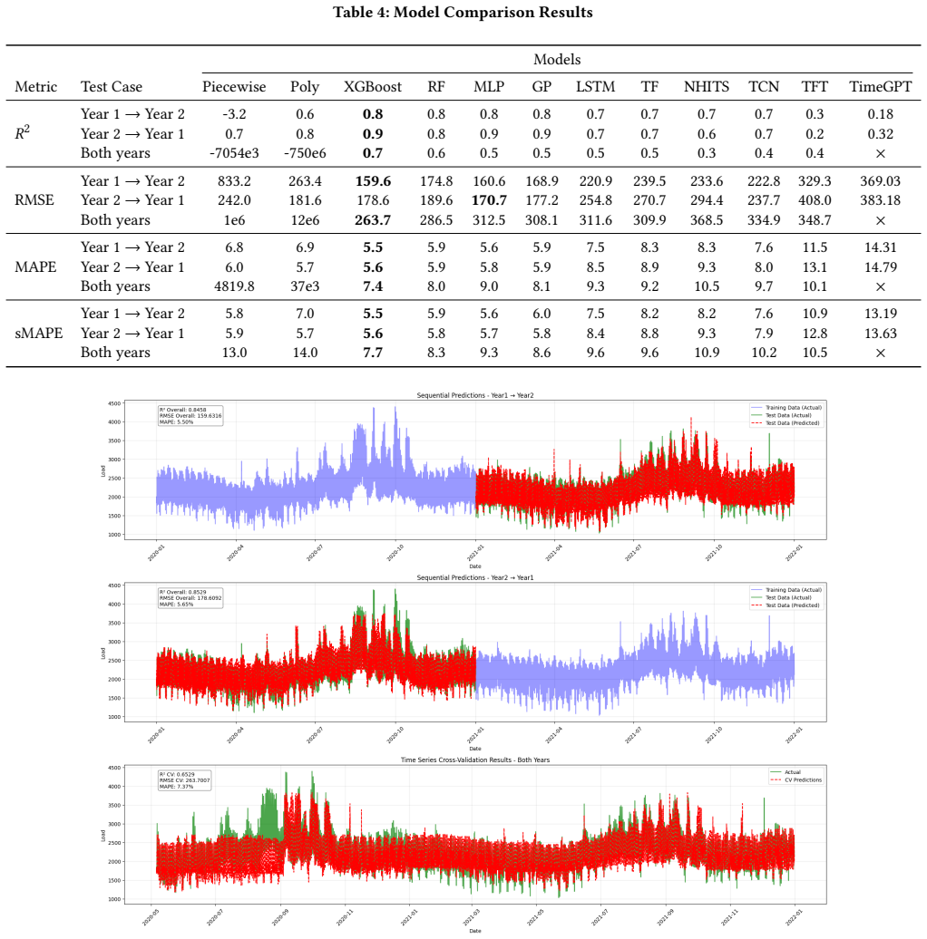
On the ESD 2025 PG&E dataset, the paper establishes that XGBoost, trained as 24 independent hourly regression models on PCA-compressed temperature and irradiance features plus calendar dummies, yields the lowest error rates across all key metrics ($R^2$, RMSE, MAPE, sMAPE) for one-day-ahead load forecasting. Deep learning architectures—including LSTM, TCN, NHITS, TFT, and the pretrained TimeGPT—fail to consistently beat simpler statistical and machine-learning baselines, which the authors attribute to limited training data, sparse exogenous variables, and error accumulation over long horizons without autoregressive updates. The final model adds a single lagged PCA exogenous feature and produces a full-year forecast with MAPE around 5.5–7.4 across test cases.
Load-bearing premise
The load-bearing premise is that the two internal test cases (predicting one training year from the other, plus five-fold cross-validation on both years) faithfully represent the undisclosed competition test year; if the hidden year's load–weather relationship differs from both training years, the XGBoost advantage may not transfer.
Editorial extensions
If this is right
- If correct, gradient-boosted tree ensembles should be the baseline of choice for day-ahead load forecasting in small-data utility settings, ahead of more complex deep architectures.
- Deep learning's failure here is not about architecture alone but about data scale and exogenous-variable availability; claims of transformer superiority need evaluation in such constrained regimes.
- Lagged and leading exogenous features add little once PCA weather and calendar features are in; instantaneous weather plus calendar largely determines load.
- The 24-hour-model stacking strategy generalizes: it can be applied to any daily-periodic forecasting task with exogenous covariates, regardless of learner.
- Computational cost arguments strengthen the case: XGBoost trains within an hour, deep models from hours to days, with no proportionate accuracy gain.
Reading between the lines
- The reported advantage rests on three internal test cases, not the undisclosed competition test; if the hidden year's weather or load regime shifts as much as Year 1 differs from Year 2, the XGBoost margin may shrink or reverse—a testable prediction once test labels are released.
- The same pipeline could be applied to other utilities or to the full ESD dataset with more sites; if the result holds broadly, it would strengthen the general claim that tree ensembles dominate deep learning in low-data load forecasting.
- The paper's framing suggests a broader principle: in time-series problems where autoregressive target lags are unavailable, decomposing by period and using strong tabular learners may outperform sequence models, because the sequence models lose their main advantage when they cannot condition on past targets.
- One could extend the work by calibrating probabilistic forecasts or by testing whether a single global model with an hour embedding matches the 24-model ensemble, a comparison not explored here.
Signed reviews
Editorial analysis
A structured set of objections, weighed in public.
Referee Report
Summary. The paper reports a case study from the IISE PG&E Energy Analytics Challenge 2025, in which the authors compare 12 forecasting models for one-day-ahead hourly electricity load prediction using two years of training data with temperature and GHI exogenous variables. The proposed framework decomposes the 24-hour forecasting task into 24 independent hourly regression models, applies PCA to the exogenous variables, and compares piecewise/polynomial regression, XGBoost, random forest, MLP, LSTM, Gaussian processes, transformers, NHITS, TCN, TFT, and TimeGPT. Based on three internal pseudo-test evaluations (Year1→Year2, Year2→Year1, and 5-fold cross-validation), the authors conclude that XGBoost delivers the lowest error rates, and they select an XGBoost variant with one lagged exogenous feature as the final model. The central claim is empirical: a gradient-boosted tree trained per hour on PCA-reduced weather covariates outperforms transformer-based and other deep learning models on MAPE and sMAPE in this constrained setting.
Significance. If the empirical ranking were established with appropriate statistical rigor, the paper would be a useful contribution to the ongoing discussion about when deep learning models, especially large pre-trained models, add value over simpler machine learning approaches in short-data, low-covariate forecasting tasks. The hourly-decomposition idea is clear and sensible, the evaluation spans many model families, and the pseudo-test setup is a reasonable attempt to approximate the hidden competition test. The main value is as a practical benchmarking case study rather than as a methodological advance. The paper explicitly credits the hourly-model inspiration to prior work, and it does not introduce a new algorithm or theoretical derivation. The strength of the contribution depends on whether the reported XGBoost advantage is robust and whether the comparison with TimeGPT is fair.
major comments (4)
- [Section 5.1, Table 4] The conclusion that 'XGBoost consistently outperforms other models across all key metrics' is not supported by the table. For Year2→Year1, MLP has lower RMSE than XGBoost (170.7 vs. 178.6), and for Year1→Year2 the XGBoost MAPE advantage over MLP is only 5.5 vs. 5.6. No error bars, confidence intervals, or paired statistical tests are reported, and the metrics are rounded to one or two decimals, so the observed margins may be within sampling noise. The abstract's claim that XGBoost 'delivers the lowest error rates across all test cases' is therefore overstated. The authors should either add significance testing or nonparametric paired comparisons, or revise the claims to describe XGBoost as competitive rather than uniformly best.
- [Appendix A, Table 4] The TimeGPT comparison appears to be run under a different protocol than the other models. Appendix A states that TimeGPT-1 used a daily loop where predictions for each day were fed into the next day's forecast, whereas the other 24 hourly models are independent regressions. This reintroduces autoregressive error accumulation for TimeGPT and makes the comparison not apples-to-apples. The statement that deep learning models, including TimeGPT, 'fail to consistently outperform' simpler approaches is load-bearing for the paper's central claim, but it is based on a model evaluated under conditions that differ from those used for XGBoost. The authors should either run TimeGPT under the same hourly-decomposition protocol or explicitly restrict the conclusion to 'under the sequential daily-loop protocol adopted for TimeGPT.'
- [Section 5.2, Table 5] The selection of Lag1 as the final model is not justified by the reported numbers. Compared with the Baseline, Lag1 has higher RMSE (Year2→Year1: 180.30 vs. 178.93), higher sMAPE (Year2→Year1: 5.68 vs. 5.61), and essentially equal MAPE on Year1→Year2 (5.55 vs. 5.54). The claimed 'slight but consistent improvements' hold only on the 'Both Years' cross-validation row, not on the two holdout-style pseudo-tests. Given that the differences are small and in both directions, the statement in Section 5.3 that Lag1 'achieves the best trade-off between accuracy and computational efficiency' needs a more explicit justification, or the paper should acknowledge that the feature-lag choice is insensitive within the reported range.
- [Section 4.3 and Section 3.1] The central empirical claim is inferred from three internal pseudo-tests, yet the hidden competition test is undisclosed. The descriptive statistics in Table 1 show that Year1 and Year2 load distributions differ substantially (e.g., standard deviation 465.77 vs. 406.48, skewness 1.18 vs. 0.67), so if the hidden year's weather or load regime differs from both training years, the reported XGBoost advantage may not transfer. The paper would be more accurate if the abstract and conclusion framed the results as evidence from internal pseudo-tests rather than as a proven statement about the actual test set. This is not a fatal flaw given the competition constraint, but the wording should be calibrated accordingly.
minor comments (5)
- [Section 4.2] The phrase 'computational efficiency and interoperability' should likely read 'interpretability,' given the earlier discussion of model interpretability.
- [Figure 4] The axes and legend of Figure 4 are not fully described in the text; adding explicit axis labels and explaining the red marks would improve readability.
- [Table 4] The '×' entry for TimeGPT on the 'Both years' cross-validation row is not explained. A footnote describing why this evaluation was not performed would prevent confusion.
- [Appendix A] The reference to 'Figure 8' states that degradation is visible 'from February to November,' but the figure does not label these months clearly; adding month labels or a short description in the caption would help.
- [References] Reference [2] is a broad survey and is cited to support deep-learning capabilities; the point would be better served by a more specific citation on transformer or attention-based load forecasting.
Circularity Check
No circularity: the XGBoost ranking is an empirical benchmark computed from ground truth, and the self-citation to the hourly-model idea is not load-bearing.
full rationale
The paper's central claim is an empirical ranking obtained by training each candidate model under the same three pseudo-test protocols (Year 1 to Year 2, Year 2 to Year 1, and 5-fold cross-validation) and comparing standard metrics. No equation in the paper defines the reported error metrics in terms of any fitted constant or model output; R^2, RMSE, MAPE, and sMAPE are computed directly from predictions and ground truth, and the regression equation y_t,h = f_h(X_t,h) + epsilon is a standard decomposition rather than a tautology. The hourly-model design is credited to Hu et al. [10], which includes a present author, but that citation supplies only a methodological template; the XGBoost victory is not derived from [10] nor forced by it, and the paper does not invoke any uniqueness theorem or ansatz from that prior work. Selecting XGBoost and Lag1 using the same pseudo-test cases that are later summarized is a potential overfitting or selection concern, not a self-definitional reduction: the reported 'lowest error' numbers are measurements on those validation cases, not predictions constructed from the fitted model's own parameters. The appendix candidly states that TimeGPT-1 was run under a different sequential protocol due to API constraints, which is a fairness issue for the comparison but not circularity. Overall, the derivation chain is self-contained: the paper's conclusions are summaries of direct empirical comparisons, not conclusions that reduce to their inputs by construction.
Assumptions & free parameters
free parameters (3)
- XGBoost hyperparameters =
not reported (Optuna search)
- PCA component count =
2 (one temperature PC, one GHI PC)
- Lag/lead feature set =
Lag1 (one lag of PCA temperature and PCA GHI)
assumptions (3)
- domain assumption The internal pseudo-test evaluations (Year1->Year2, Year2->Year1, 5-fold CV) are predictive of performance on the hidden test year.
- domain assumption The underlying calendar years are 2020, 2021, and 2022.
- domain assumption Exogenous variables available day-ahead (temperature and GHI) contain enough signal to predict hourly load without lagged load values.
Cite this review
Pith. "Pith review of IISE PG&E Energy Analytics Challenge 2025: Hourly-Binned Regression Models Beat Transformers in Load Forecasting." pith.science (2026). https://pith.science/paper/67ENQWIL
@misc{pith2026250511390,
  author       = {Pith},
  title        = {Pith review of: IISE PG&E Energy Analytics Challenge 2025: Hourly-Binned Regression Models Beat Transformers in Load Forecasting},
  year         = {2026},
  howpublished = {\url{https://pith.science/paper/67ENQWIL}},
  note         = {Machine review of arXiv:2505.11390}
}
read the original abstract
Accurate electricity load forecasting is essential for grid stability, resource optimization, and renewable energy integration. While transformer-based deep learning models like TimeGPT have gained traction in time-series forecasting, their effectiveness in long-term electricity load prediction remains uncertain. This study evaluates forecasting models ranging from classical regression techniques to advanced deep learning architectures using data from the ESD 2025 competition. The dataset includes two years of historical electricity load data, alongside temperature and global horizontal irradiance (GHI) across five sites, with a one-day-ahead forecasting horizon. Since actual test set load values remain undisclosed, leveraging predicted values would accumulate errors, making this a long-term forecasting challenge. We employ (i) Principal Component Analysis (PCA) for dimensionality reduction and (ii) frame the task as a regression problem, using temperature and GHI as covariates to predict load for each hour, (iii) ultimately stacking 24 models to generate yearly forecasts. Our results reveal that deep learning models, including TimeGPT, fail to consistently outperform simpler statistical and machine learning approaches due to the limited availability of training data and exogenous variables. In contrast, XGBoost, with minimal feature engineering, delivers the lowest error rates across all test cases while maintaining computational efficiency. This highlights the limitations of deep learning in long-term electricity forecasting and reinforces the importance of model selection based on dataset characteristics rather than complexity. Our study provides insights into practical forecasting applications and contributes to the ongoing discussion on the trade-offs between traditional and modern forecasting methods.
Figures


Figures from the paper (4 more)


Reference graph
Works this paper leans on
-
[10]
Yinbo Hu, Michael Waite, Evan Patz, Bainan Xia, Yixing Xu, Daniel Olsen, Naveen Gopan, and Vijay Modi. A data-driven approach for the disaggregation of building-sector heating and cooling loads from hourly utility load data. En- ergy Strategy Reviews, 49:101175, 2023
work page 2023
-
[1]
Probabilistic time series forecast- ing with recurrent neural networks for intermittent demand
Mariana Arias Chao and Volodymyr Kuleshov. Probabilistic time series forecast- ing with recurrent neural networks for intermittent demand. IEEE Transactions on Neural Networks and Learning Systems , 33(6):2620–2631, 2022
work page 2022
-
[2]
Neural forecasting: Introduction and literature overview
Konstantinos Benidis, Syama Sundar Rangapuram, Valentin Flunkert, Bernie Wang, Danielle Maddix, Caner Turkmen, Jan Gasthaus, Michael Bohlke-Schneider, David Salinas, Lorenzo Stella, et al. Neural forecasting: Introduction and literature overview. arXiv preprint arXiv:2004.10240, 2020
arXiv 2004
-
[3]
Mapping properties of Fourier transforms, revisited
Wei Chen, Jingyu Chen, and Jianmin Zhang. Gpt4ts: Prompt learning for time series forecasting. arXiv preprint arXiv:2310.13567, 2023. 8 Figure 7: Final Forecast by Month Figure 8: Long-Horizon TimeGPT-1 Forecasting
work page Pith review arXiv 2023
-
[4]
Tsfpaper: A reposi- tory of time series forecasting papers
Dongzhe Du, Wei Chen, Xiuwen Wang, and Jianmin Zhang. Tsfpaper: A reposi- tory of time series forecasting papers. https://github.com/ddz16/TSFpaper, 2023. Accessed: 2025-03-20
work page 2023
-
[5]
Staff report on data needs for electricity system planning
Federal Energy Regulatory Commission. Staff report on data needs for electricity system planning. Staff report, FERC, 2021
work page 2021
-
[6]
The m4 forecasting competition—a practitioner’s view
Michael Gilliland. The m4 forecasting competition—a practitioner’s view. Inter- national Journal of Forecasting , 35(1):161–174, 2019
work page 2019
-
[7]
Monash time series forecasting archive
Rakshitha Godahewa, Christoph Bergmeir, Geoffrey I Webb, Rob J Hyndman, and Pablo Montero-Manso. Monash time series forecasting archive. arXiv preprint arXiv:2105.06643, 2021. 9
arXiv 2021
Show all 37 references
-
[8]
Simple versus complex forecasting: The evidence
Kesten C Green and J Scott Armstrong. Simple versus complex forecasting: The evidence. Journal of Business Research , 68(8):1678–1685, 2015
2015
-
[9]
Analysis and clustering of residential customers energy behavioral patterns using robust data mining techniques
Stephen Haben, Colin Singleton, and Peter Grindrod. Analysis and clustering of residential customers energy behavioral patterns using robust data mining techniques. International Journal of Forecasting , 32(3):717–730, 2016
2016
-
[11]
Large-scale unusual time series detection
Rob J Hyndman, Earo Wang, and Nikolay Laptev. Large-scale unusual time series detection. In IEEE International Conference on Data Mining Workshops (ICDMW) , pages 1616–1619, 2020
2020
-
[12]
Criteria for classifying forecasting methods
Tim Januschowski, Jan Gasthaus, Yuyang Wang, David Salinas, Valentin Flunkert, Michael Bohlke-Schneider, and Laurent Callot. Criteria for classifying forecasting methods. International Journal of Forecasting , 36(1):167–177, 2020
2020
-
[13]
Renewable Energy-Storage Systems Integration in Power Grids: Modeling, Control and Optimization
Chongqing Kang, Ning Zhang, Qing Xia, and Yi Ding. Renewable Energy-Storage Systems Integration in Power Grids: Modeling, Control and Optimization. Academic Press, 2020
2020
-
[14]
Extended forecast methods for day-ahead electricity spot prices applying artificial neural networks
Dogan Keles, Jonathan Scelle, Florentina Paraschiv, and Wolf Fichtner. Extended forecast methods for day-ahead electricity spot prices applying artificial neural networks. Applied Energy, 162:218–230, 2016
2016
-
[15]
Forecasting spot electricity prices: Deep learning approaches and empirical comparison of traditional algorithms
Jesus Lago, Fjo De Ridder, and Bart De Schutter. Forecasting spot electricity prices: Deep learning approaches and empirical comparison of traditional algorithms. Applied Energy, 221:386–405, 2018
2018
-
[16]
Modeling long- and short-term temporal patterns with deep neural networks
Guokun Lai, Wei-Cheng Chang, Yiming Yang, and Hanxiao Liu. Modeling long- and short-term temporal patterns with deep neural networks. In The 41st Interna- tional ACM SIGIR Conference on Research & Development in Information Retrieval , pages 95–104, 2018
2018
-
[17]
Renewable energy and demand forecasting in an integrated smart grid
Vishnu Vardhan Sai Lanka, Millend Roy, Shikhar Suman, and Shivam Prajapati. Renewable energy and demand forecasting in an integrated smart grid. In 2021 Innovations in Energy Management and Renewable Resources(52042) , pages 1–6, 2021
2021
-
[18]
Deep learning for electricity market forecasting: Current methods, challenges and opportunities
Miguel Legault, Alexandre Ouellet, Gaelle Saint-Hilary, Mathilde Bourdeau, and Barthelemy Ateme-Nguema. Deep learning for electricity market forecasting: Current methods, challenges and opportunities. Renewable and Sustainable Energy Reviews, 168:112778, 2022
2022
-
[19]
Efficiently modeling long sequences with structured state spaces
Albert Q Li, Tri Dao, Bryan Lim, Philip Lichtarge, Sercan O Arik, Michael Y Li, and Tomas Pfister. Efficiently modeling long sequences with structured state spaces. arXiv preprint arXiv:2111.00396, 2022
2022 arXiv
-
[20]
Temporal fusion transformers for interpretable multi-horizon time series forecasting.International Journal of Forecasting, 37(4):1748–1764, 2021
Bryan Lim, Sercan O Arık, Nicolas Loeff, and Tomas Pfister. Temporal fusion transformers for interpretable multi-horizon time series forecasting.International Journal of Forecasting, 37(4):1748–1764, 2021
2021
-
[21]
Statistical and machine learning forecasting methods: Concerns and ways forward
Spyros Makridakis, Evangelos Spiliotis, and Vassilios Assimakopoulos. Statistical and machine learning forecasting methods: Concerns and ways forward. PloS one, 13(3):e0194889, 2018
2018
-
[22]
The m5 competition: Background, organization, and implementation.International Journal of Forecasting, 38(4):1325– 1336, 2022
Spyros Makridakis, Evangelos Spiliotis, Vassilios Assimakopoulos, Zhi Chen, Anil Gaba, Ilia Tsetlin, and Robert L Winkler. The m5 competition: Background, organization, and implementation.International Journal of Forecasting, 38(4):1325– 1336, 2022
2022
-
[23]
Fforma: Feature-based forecast model averaging
Pablo Montero-Manso, George Athanasopoulos, Rob J Hyndman, and Thiyanga S Talagala. Fforma: Feature-based forecast model averaging. International Journal of Forecasting, 36(1):86–92, 2020
2020
-
[24]
Reliability guideline: Methods for establishing resource adequacy requirements
North American Electric Reliability Corporation. Reliability guideline: Methods for establishing resource adequacy requirements. Technical report, NERC, 2022
2022
-
[25]
Computing electricity spot price predic- tion intervals using quantile regression and forecast averaging
Jakub Nowotarski and Rafal Weron. Computing electricity spot price predic- tion intervals using quantile regression and forecast averaging. Computational Statistics, 30(3):791–803, 2013
2013
-
[26]
N-beats: Neural basis expansion analysis for interpretable time series forecasting
Boris N Oreshkin, Dmitri Carpov, Nicolas Chapados, and Yoshua Bengio. N-beats: Neural basis expansion analysis for interpretable time series forecasting. arXiv preprint arXiv:1905.10437, 2020
1905 arXiv
-
[27]
Forecasting: theory and practice
Fotios Petropoulos, Daniele Apiletti, Vassilios Assimakopoulos, Mohamed Zied Babai, Devon K Barrow, Souhaib Ben Taieb, Christoph Bergmeir, Ricardo J Bessa, Jakub Bijak, John E Boylan, et al. Forecasting: theory and practice. International Journal of Forecasting, 38(3):705–871, 2022
2022
-
[28]
Deep state space models for time series forecasting
Syama Sundar Rangapuram, Matthias W Seeger, Jan Gasthaus, Lorenzo Stella, Yuyang Wang, and Tim Januschowski. Deep state space models for time series forecasting. Advances in neural information processing systems , 31, 2018
2018
-
[29]
Probabilistic load forecasting for large-scale distributed energy resources aggregation
Jakub Rubaszewski, Jakub Nowotarski, and Rafal Weron. Probabilistic load forecasting for large-scale distributed energy resources aggregation. IEEE Trans- actions on Smart Grid , 13(3):2133–2146, 2022
2022
-
[30]
Machine learning based adaptive fault diagnosis consid- ering hosting capacity amendment in active distribution network
Sourav Kumar Sahu, Millend Roy, Soham Dutta, Debomita Ghosh, and Dus- manta Kumar Mohanta. Machine learning based adaptive fault diagnosis consid- ering hosting capacity amendment in active distribution network. Electric Power Systems Research, 216:109025, 2023
2023
-
[31]
Deepar: Probabilistic forecasting with autoregressive recurrent networks
David Salinas, Valentin Flunkert, Jan Gasthaus, and Tim Januschowski. Deepar: Probabilistic forecasting with autoregressive recurrent networks. International Journal of Forecasting, 36(3):1181–1191, 2020
2020
-
[32]
Financial time series forecasting with deep learning: A systematic literature review: 2005–
Omer Berat Sezer, Mehmet Ugur Gudelek, and Ahmet Murat Ozbayoglu. Financial time series forecasting with deep learning: A systematic literature review: 2005–
2005
-
[33]
Review of smart meter data analytics: Applications, methodologies, and challenges
Yi Wang, Qixin Chen, Tao Hong, and Chongqing Kang. Review of smart meter data analytics: Applications, methodologies, and challenges. IEEE Transactions on Smart Grid, 10(3):3125–3148, 2019
2019
-
[34]
Electricity price forecasting: A review of the state-of-the-art with a look into the future
Rafal Weron. Electricity price forecasting: A review of the state-of-the-art with a look into the future. International Journal of Forecasting , 30(4):1030–1081, 2014
2014
-
[35]
Autoformer: De- composition transformers with auto-correlation for long-term series forecasting
Haixu Wu, Jiehui Xu, Jianmin Wang, and Mingsheng Long. Autoformer: De- composition transformers with auto-correlation for long-term series forecasting. Advances in Neural Information Processing Systems , 34:22419–22430, 2021
2021
-
[36]
all-at-once
Tian Zhou, Ziqing Ma, Qingsong Wen, Xue Wang, Liang Sun, and Rong Jin. Fedformer: Frequency enhanced decomposed transformer for long-term series forecasting. In International Conference on Machine Learning , pages 41269–41286, 2023. A Discussions on TimeGPT Short-Horizon Forec...
2023
-
[2019]
Applied Soft Computing, 90:106181, 2020
2020
Reviewed August 15, 2026 · model on record in the stance chip above.
Discussion (0). Continue with ORCID to comment.