REVIEW 3 major objections 5 minor 49 references
The paper shows that in a log-strain viscoelastic model, the polymer-to-solvent viscosity ratio independently controls how strongly non-Newtonian flow profiles develop with increasing Weissenberg number, and that the model cannot be reduced
Reviewed by Pith at T0; open to challenge. T0 means a machine referee read the full paper against a public rubric. the ladder, T0–T4 →
2026-08-04 18:05 UTC pith:6K5GLNPG
load-bearing objection First FE benchmarks for the log-strain model with a credible ξ–Wi story, but the claimed enforcement of positive definiteness isn't in the equations. the 3 major comments →
A numerical study to analyze the interplay of Weissenberg number and viscosity ratio in a log-strain tensorial model for viscoelastic fluids
The pith
A machine-rendered reading of the paper's core claim, the machinery that carries it, and where it could break.
Core claim
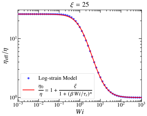
The central claim, on the paper's own terms, is that the Weissenberg number and the viscosity ratio xi = kappa*tau_r/eta play independent roles in the log-strain model, with xi determining the extent to which raising Wi produces observably non-Newtonian behavior. In straight-channel flow the profiles interpolate between the solvent-only and zero-shear Newtonian limits, developing a plug-like central region at intermediate Wi that shrinks as Wi grows; this plug-like regime requires sufficiently large xi. In flow past a cylinder the drag coefficient transitions from the zero-shear to the solvent baseline as the effective strain rate rises. In the 4:1 contraction the corner vortex size varies n
What carries the argument
The central object is the elastic strain tensor Bel, a symmetric positive definite tensor with unit determinant that plays the role of a conformation tensor; its evolution is the upper-convected derivative of Bel balanced by the relaxation term -(1/tau_r) Bel*log(Bel), and the elastic stress is Tel = kappa*log(Bel). The independent dimensionless parameter xi = kappa*tau_r/eta, the ratio of polymeric to solvent viscosity contributions, is the knob that controls how much shear thinning the model displays. The computational machinery is a staggered semi-implicit time-stepping scheme using a generalized Lie derivative with semi-Lagrangian advection for the strain update, a Variational Multiscale
Load-bearing premise
The simulations assume that the computed elastic strain tensor Bel stays symmetric positive definite with unit determinant; the code's projection enforces only symmetry and unit determinant, not positive eigenvalues, so the physical validity of the reported solutions depends on an unverified positivity property.
What would settle it
Check the computed Bel field in any of the reported runs for points where the symmetrized tensor has a non-positive determinant or a negative eigenvalue. The existence of even one such point would mean the asserted preservation of positive definiteness does not hold in the discretization, and the steady states reported at high Wi may reflect the projection's repair rather than the log-strain model's dynamics.
If this is right
- In straight-channel pressure-driven flow, increasing xi at fixed Wi turns the parabolic velocity profile into a plug-like shear-thinning profile with a central plug region that shrinks as Wi grows; at small xi the profile stays nearly parabolic for all Wi.
- In flow past a cylinder, the drag coefficient drops from the zero-shear Newtonian baseline toward the solvent-only baseline as the effective strain rate increases, with the magnitude of the reduction set by xi.
- In the 4:1 planar contraction at large xi, the corner vortex size changes non-monotonically with Wi and no secondary lip vortex appears, in line with strongly shear-thinning behavior.
- A Generalized Newtonian Fluid fitted to the simple-shear viscosity of the log-strain model reproduces the channel-flow profile to within a few percent but fails around the cylinder, where extensional deformation makes the log-strain model more dissipative; the model is therefore not equivalent to a shear-rate-dependent viscosity.
- The stabilized formulation sustains steady-state computations up to Wi around 35 in these benchmark geometries, beyond the typical limit of many unstabilized viscoelastic formulations.
Where Pith is reading between the lines
- If this xi-dependence persists in other geometries, then reporting the Weissenberg number alone is insufficient: experiments and simulations should quote the viscosity ratio as well, or the same Wi can correspond to qualitatively different flow fields.
- The mismatch between the log-strain and Generalized Newtonian solutions in mixed shear/extension flows could serve as a quantitative probe of flow-type-dependent rheology, potentially distinguishing this model from purely shear-thinning constitutive equations in microfluidic experiments.
- A direct way to test the numerical enforcement claim is to record the eigenvalues of Bel during the simulations; if positivity is ever lost locally, the high-Wi results would be artifacts of the projection step rather than predictions of the model.
- The predicted absence of secondary lip vortices in the 4:1 contraction could be used experimentally to distinguish strongly shear-thinning log-strain behavior from constant-viscosity viscoelastic models that typically produce lip vortices.
Editorial analysis
A structured set of objections, weighed in public.
Referee Report
Summary. The manuscript reports a numerical study of the log-strain viscoelastic model of Alrashdi and Giusteri, focusing on the separate roles of the Weissenberg number Wi and the viscosity ratio ξ = κτ_r/η. A stabilized mixed finite element method (equal-order P1-P1 with VMS stabilization and a DG0 strain field) is combined with a backward-Euler/semi-Lagrangian treatment of the upper-convected derivative. The method is applied to three benchmark flows: straight channel, flow past a cylinder, and 4:1 planar contraction. The authors find that ξ controls the degree of shear-thinning and hence the appearance of plug-like profiles, that drag reduction occurs in cylinder flow, that no lip vortices appear in the contraction, and that the model cannot be reduced to a Generalized Newtonian Fluid: comparing the log-strain model with a GNF model fitted to the same simple-shear effective viscosity, they report significant profile differences in the cylinder flow that they attribute to flow-type dependence.
Significance. If the numerical results are reliable, the paper makes a useful contribution by demonstrating that Wi and ξ are independent control parameters for the log-strain model and that the model's behavior in non-viscometric flows is not captured by a shear-rate-dependent viscosity alone. The GNF comparison is a good way to isolate flow-type effects, and reaching Wi ~ 35 with a relatively new tensorial model is a practical achievement. However, the paper's central numerical-verification claim is not supported: the projection used in the discrete update does not enforce positive definiteness, and mesh/time-convergence evidence is only qualitative. The physical conclusions are therefore conditional on additional verification.
major comments (3)
- [Section 3.1, Eq. (18)] The abstract and Section 3.1 state that the computational method enforces symmetry, unit determinant, and positive definiteness of B_el. The projection in Eq. (18) only symmetrizes the tensor and rescales it to unit determinant. A symmetric 2x2 matrix with eigenvalues (-1,-1) has determinant 1 but is negative definite, and Eq. (18) leaves it unchanged. If det(sym(B)) ≤ 0 the projection is undefined. Since Eq. (17) requires log B_el^n, loss of positive definiteness makes the evolution ill-defined and the subsequent results non-physical. The manuscript reports no check on the minimum eigenvalue of B_el. This is load-bearing because all reported flow fields and the GNF comparison depend on the computed B_el being admissible. The authors should either prove that the discrete update plus projection preserves positive definiteness under the conditions used, or add numerical monitoring of the s
- [Section 4 (general numerical verification)] Mesh convergence is asserted qualitatively: Section 4.1.1 states a 64x64 mesh is 'sufficient', and Sections 4.2.1 and 4.3.1 state that convergence was 'verified through successive refinements' without quantitative tables or error norms. Similarly, steady state is defined by increment norms decaying to 'machine precision', but no tolerance, history, or time-step dependence is reported. For a numerical study that reaches Wi ~ 35 and includes a re-entrant corner singularity, quantitative mesh-convergence and time-step studies are necessary to support the reliability of the reported steady-state fields. Please add tables or figures with grid sizes, L2 error norms or Richardson extrapolation, and the convergence history of the increment norms.
- [Section 4.4, Figures 11-12] The central claim that flow-type dependence is significant in the cylinder flow rests on comparing the log-strain model with a GNF model whose viscosity is an approximate Cross fit (β = 0.788, n = 1.458). The authors acknowledge a mismatch in the intermediate shear-rate region and attribute the 2.63% channel profile discrepancy to it. In the cylinder flow, they argue that the profile differences are not a mere scaling and hence cannot be due to fitting error. This is suggestive but not conclusive: a local shear-rate error in the GNF model could produce shape changes in a non-unidirectional flow. To make the identification robust, the comparison should be repeated using the exact tabulated effective viscosity from the log-strain model in simple shear, or the sensitivity of the cylinder profiles to plausible variations of β and n should be quantified.
minor comments (5)
- [Figure 7] The axis/panel labels appear garbled ('b=25' and '8=...' instead of ξ and Wi). Please check the figure rendering.
- [Figure 9] The legend in panel (b) repeats the entry 'Wi=0.0, C=10.0' twice; one of the entries should be a different Newtonian reference (e.g., C=15.0).
- [Section 3.1] The hat notation is used in Eq. (14) before it is defined after Eq. (20). Define the notation earlier.
- [Section 4.4.1] The Cross fit parameters β and n are given without confidence intervals or a goodness-of-fit measure. Given the importance of the fit to the GNF comparison, report at least one measure such as R² or the mean relative error.
- [Data availability] The code and data are only available 'on request'. For a numerical study of this type, a public repository with the FEniCSx scripts would substantially strengthen reproducibility.
Circularity Check
No significant circularity: the GNF comparison is a fitted surrogate used only as a baseline, and the main numerical conclusions are independent simulations of the stated model.
full rationale
The paper is a numerical study of a constitutive model introduced in [23] by one of the authors. The central claims — that the viscosity ratio ξ modulates the extent to which Wi produces non-Newtonian profiles, and that the log-strain model differs from a Generalized Newtonian Fluid surrogate in a flow with extensional character — are obtained by solving the stated model equations (6)–(8) for specified parameters. No parameter appearing in the reported velocity profiles or drag coefficients is fitted to those target outputs: ξ is set by κτr/η (Eq. 9), Wi by Uτr/L, and the Cross parameters β,n in Eq. (44) are fitted only to the log-strain model's own steady simple-shear effective viscosity (Eq. 43) to build the comparison GNF model. That is a controlled surrogate construction, not a hidden prediction of the target results. The differences between log-strain and GNF in cylinder flow are argued from non-scaling profile shapes, not from the fitted values. Citations to the authors' earlier paper [23] introduce the model and its linearized limits, but the quantitative results here are independent simulations and do not reduce to those citations. The projection in Eq. (18) may fail to enforce positive definiteness, but that is a numerical correctness concern, not circularity: it does not make an output equal to an input. No definitional reduction, fitted-input-as-prediction, or self-citation chain forces the conclusions.
Axiom & Free-Parameter Ledger
free parameters (3)
- Cross model time constant β =
0.788
- Cross model power-law exponent n =
1.458
- VMS stabilization constants c1, c2 =
c1 = 4k^4, c2 = 2k^2 (k = 1 for P1)
axioms (5)
- domain assumption The log-strain constitutive equations (6)-(8) correctly describe the viscoelastic fluid and preserve det Bel = 1, symmetry, and positive definiteness.
- domain assumption A steady state exists for each simulated parameter set and is reached by time marching to machine-precision increment norms.
- domain assumption The semi-Lagrangian characteristic mapping (Eq. 17) is a consistent and sufficiently stable discretization of the upper-convected Lie derivative.
- domain assumption The VMS stabilization with parameters α1 and α2 defined in Eq. (29), using c1 = 4k^4 and c2 = 2k^2, yields a stable and converged discretization for the tested regimes.
- domain assumption The discrete update plus projection (18) keeps Bel in the physically admissible set of symmetric positive definite tensors with determinant 1.
Cite this review
Pith. "Pith review of A numerical study to analyze the interplay of Weissenberg number and viscosity ratio in a log-strain tensorial model for viscoelastic fluids." pith.science (2026). https://pith.science/paper/6K5GLNPG
@misc{pith2026260801925,
  author       = {Pith},
  title        = {Pith review of: A numerical study to analyze the interplay of Weissenberg number and viscosity ratio in a log-strain tensorial model for viscoelastic fluids},
  year         = {2026},
  howpublished = {\url{https://pith.science/paper/6K5GLNPG}},
  note         = {Machine review of arXiv:2608.01925}
}
read the original abstract
We present a computational study aimed at exploring the different and independent roles of the Weissenberg number and of the ratio between the polymeric and solvent viscosity contributions in a viscoelastic fluid model. The tensorial model under investigation, recently proposed, is based on a logarithmic relation between the elastic (or recoverable) strain and the elastic stress. In this model, the elastic strain plays the role of a conformation tensor and its evolution equation inherently preserves its determinant and positive definiteness. These properties are also enforced in the computational method employed in the study. A finite-difference discretization in time is combined with a stabilized mixed finite element formulation based on the Variational Multiscale method for the spatial discretization and with a generalized Lie derivative approach for the advection terms. The behavior of the model is analyzed in paradigmatic pressure-driven flows and we find that the value of the viscosity ratio is crucial in determining to which extent non-Newtonian flow profiles are observed upon increasing the Weissenberg number. By comparing the solutions of the log-strain tensorial model with those of a suitable Generalized Newtonian Fluid model, we show that flow-type dependence plays a significant role even in the simple planar flow past a cylinder.
Figures




Reference graph
Works this paper leans on
-
[1]
M. D. Graham, Drag reduction in turbulent flow of polymer solutions, Rheology reviews 2 (2004) 143–170
2004
-
[2]
Groisman, V
A. Groisman, V. Steinberg, Elastic turbulence in a polymer solution flow, Nature 405 (2000) 53–55
2000
-
[3]
S. S. Datta, A. M. Ardekani, P. E. Arratia, A. N. Beris, I. Bischofberger, G. H. McKinley, J. G. Eggers, J. E. López-Aguilar, S. M. Fielding, A. Frishman, et al., Perspectives on viscoelastic flow instabilities and elastic turbulence, Physical Review Fluids 7 (2022) 080701
2022
-
[4]
H. A. C. Sánchez, M. R. Jovanović, S. Kumar, A. Morozov, V. Shankar, G. Subramanian, H. J. Wilson, Understanding viscoelastic flow instabilities: Oldroyd-B and beyond, Journal of Non- Newtonian Fluid Mechanics 302 (2022) 104742
2022
-
[5]
J. G. Oldroyd, On the formulation of rheological equations of state, Proceedings of the Royal Society of London. Series A. Mathematical and Physical Sciences 200 (1950) 523–541
1950
-
[6]
Oldroyd, Non-newtonian effects in steady motion of some idealized elastico-viscous liquids, Proceedings of the Royal Society of London
J. Oldroyd, Non-newtonian effects in steady motion of some idealized elastico-viscous liquids, Proceedings of the Royal Society of London. Series A. Mathematical and Physical Sciences 245 (1958) 278–297
1958
-
[7]
Giesekus, Die elastizität von flüssigkeiten, Rheologica Acta 5 (1966) 29–35
H. Giesekus, Die elastizität von flüssigkeiten, Rheologica Acta 5 (1966) 29–35. 21
1966
-
[8]
H. Giesekus, A simple constitutive equation for polymer fluids based on the concept of deformation-dependent tensorial mobility, Journal of Non-Newtonian Fluid Mechanics 11 (1982) 69–109
1982
-
[9]
Phan-Thien, R
N. Phan-Thien, R. I. Tanner, A new constitutive equation derived from network theory, Journal of Non-Newtonian Fluid Mechanics 2 (1977) 353–365
1977
-
[10]
Fattal, R
R. Fattal, R. Kupferman, Constitutive laws for the matrix-logarithm of the conformation tensor, Journal of Non-Newtonian Fluid Mechanics 123 (2004) 281–285
2004
-
[11]
Balci, B
N. Balci, B. Thomases, M. Renardy, C. R. Doering, Symmetric factorization of the conformation tensor in viscoelastic fluid models, Journal of Non-Newtonian Fluid Mechanics 166 (2011) 546– 553
2011
-
[12]
Afonso, F
A. Afonso, F. Pinho, M. Alves, The kernel-conformation constitutive laws, Journal of Non- Newtonian Fluid Mechanics 167 (2012) 30–37
2012
-
[13]
R. B. Bird, R. C. Armstrong, O. Hassager, Dynamics of polymeric liquids. Vol. 1: Fluid mechanics, John Wiley and Sons Inc., New York, NY, 1986
1986
-
[14]
Phan-Thien, Understanding viscoelasticity: An introduction to rheology, Applied Rheology 13 (2003) 240–241
N. Phan-Thien, Understanding viscoelasticity: An introduction to rheology, Applied Rheology 13 (2003) 240–241
2003
-
[15]
Alves, P
M. Alves, P. Oliveira, F. Pinho, Numerical methods for viscoelastic fluid flows, Annual Review of Fluid Mechanics 53 (2021) 509–541
2021
-
[16]
M.V.Shitikova, A.I.Krusser, Modelsofviscoelasticmaterials: areviewonhistoricaldevelopment and formulation, Theoretical Analyses, Computations, and Experiments of Multiscale Materials: A Tribute to Francesco dell’Isola (2022) 285–326
2022
-
[17]
Renardy, Recent advances in the mathematical theory of steady flow of viscoelastic fluids, Journal of Non-Newtonian Fluid Mechanics 29 (1988) 11–24
M. Renardy, Recent advances in the mathematical theory of steady flow of viscoelastic fluids, Journal of Non-Newtonian Fluid Mechanics 29 (1988) 11–24
1988
-
[18]
J. Zhou, I. Papautsky, Viscoelastic microfluidics: Progress and challenges, Microsystems & Nanoengineering 6 (2020) 113
2020
-
[19]
Renardy, B
M. Renardy, B. Thomases, A mathematician’s perspective on the Oldroyd-B model: progress and future challenges, Journal of Non-Newtonian Fluid Mechanics 293 (2021) 104573
2021
-
[20]
A. N. Beris, Continuum mechanics modeling of complex fluid systems following Oldroyd’s seminal 1950 work, Journal of Non-Newtonian Fluid Mechanics 298 (2021) 104677
1950
-
[21]
P. S. Stephanou, V. G. Mavrantzas, G. C. Georgiou, Continuum model for the phase behavior, microstructure, and rheology of unentangled polymer nanocomposite melts, Macromolecules 47 (2014) 4493–4513
2014
-
[22]
Ferrás, M
L. Ferrás, M. Morgado, M. Rebelo, G. H. McKinley, A. Afonso, A generalised Phan– Thien—Tanner model, Journal of Non-Newtonian Fluid Mechanics 269 (2019) 88–99
2019
-
[23]
M.A.H.Alrashdi, G.G.Giusteri, Evolutionoflocalrelaxedstatesandthemodelingofviscoelastic fluids, Physics of Fluids 36 (2024)
2024
-
[24]
R. G. Owens, T. N. Phillips, Computational rheology, World Scientific, 2002
2002
-
[25]
Hulsen, A
M. Hulsen, A. Van Heel, B. Van Den Brule, Simulation of viscoelastic flows using brownian configuration fields, Journal of Non-Newtonian Fluid Mechanics 70 (1997) 79–101. 22
1997
-
[26]
Fattal, R
R. Fattal, R. Kupferman, Time-dependent simulation of viscoelastic flows at high weissenberg number using the log-conformation representation, Journal of Non-Newtonian Fluid Mechanics 126 (2005) 23–37
2005
-
[27]
M. A. Hulsen, R. Fattal, R. Kupferman, Flow of viscoelastic fluids past a cylinder at high weissenberg number: stabilized simulations using matrix logarithms, Journal of Non-Newtonian Fluid Mechanics 127 (2005) 27–39
2005
-
[28]
O. M. Coronado, D. Arora, M. Behr, M. Pasquali, A simple method for simulating general viscoelastic fluid flows with an alternate log-conformation formulation, Journal of Non-Newtonian Fluid Mechanics 147 (2007) 189–199
2007
-
[29]
Advances in Stabilized Methods in Computational Mechanics
T.J.Hughes, G.R.Feijóo, L.Mazzei, J.-B.Quincy, Thevariationalmultiscalemethod–aparadigm for computational mechanics, Computer Methods in Applied Mechanics and Engineering 166 (1998) 3–24. Advances in Stabilized Methods in Computational Mechanics
1998
-
[30]
R. Codina, Stabilization of incompressibility and convection through orthogonal sub-scales in finite element methods, Computer methods in applied mechanics and engineering 190 (2000) 1579–1599
2000
-
[31]
R. Codina, Stabilized finite element approximation of transient incompressible flows using orthog- onal subscales, Computer methods in applied mechanics and engineering 191 (2002) 4295–4321
2002
-
[32]
Codina, Analysis of a stabilized finite element approximation of the oseen equations using orthogonal subscales, Applied Numerical Mathematics 58 (2008) 264–283
R. Codina, Analysis of a stabilized finite element approximation of the oseen equations using orthogonal subscales, Applied Numerical Mathematics 58 (2008) 264–283
2008
-
[33]
Castillo, R
E. Castillo, R. Codina, Stabilized stress–velocity–pressure finite element formulations of the Navier–Stokes problem for fluids with non-linear viscosity, Computer methods in applied me- chanics and engineering 279 (2014) 554–578
2014
-
[34]
Castillo, R
E. Castillo, R. Codina, Variational multi-scale stabilized formulations for the stationary three- field incompressible viscoelastic flow problem, Computer Methods in Applied Mechanics and Engineering 279 (2014) 579–605
2014
-
[35]
Castillo, R
E. Castillo, R. Codina, Numerical analysis of a stabilized finite element approximation for the three-field linearized viscoelastic fluid problem using arbitrary interpolations, ESAIM: Mathe- matical Modelling and Numerical Analysis 51 (2017) 1407–1427
2017
-
[36]
G. R. Barrenechea, E. Castillo, R. Codina, Time-dependent semidiscrete analysis of the vis- coelastic fluid flow problem using a variational multiscale stabilized formulation, IMA Journal of Numerical Analysis 39 (2019) 792–819
2019
-
[37]
Kwack, A
J. Kwack, A. Masud, A three-field formulation for incompressible viscoelastic fluids, International Journal of Engineering Science 48 (2010) 1413–1432
2010
-
[38]
Kwack, A
J. Kwack, A. Masud, K. Rajagopal, Stabilized mixed three-field formulation for a generalized incompressible Oldroyd-B model, International Journal for Numerical Methods in Fluids 83 (2017) 704–734
2017
-
[39]
D. D. Medeiros, H. Notsu, C. M. Oishi, Second-order finite difference approximations of the upper-convected time derivative, SIAM Journal on Numerical Analysis 59 (2021) 2955–2988
2021
-
[40]
B. S. Ashby, T. Pryer, Discretisation of an Oldroyd-B viscoelastic fluid flow using a lie derivative formulation, Advances in Computational Mathematics 51 (2025) 1
2025
-
[41]
Y.-J. Lee, J. Xu, C.-S. Zhang, Global existence, uniqueness and optimal solvers of discretized viscoelastic flow models, Mathematical Models and Methods in Applied Sciences 21 (2011) 1713– 1732. 23
2011
-
[42]
Y.-J. Lee, J. Xu, New formulations, positivity preserving discretizations and stability analysis for non-Newtonian flow models, Computer methods in applied mechanics and engineering 195 (2006) 1180–1206
2006
-
[43]
Y.-J. Lee, J. Xu, C.-S. Zhang, Stable finite element discretizations for viscoelastic flow models, in: Handbook of numerical analysis, volume 16, Elsevier, 2011, pp. 371–432
2011
-
[44]
T. J. Hughes, G. R. Feijóo, L. Mazzei, J.-B. Quincy, The variational multiscale method—a paradigm for computational mechanics, Computer methods in applied mechanics and engineering 166 (1998) 3–24
1998
-
[45]
Moreno, R
L. Moreno, R. Codina, J. Baiges, E. Castillo, Logarithmic conformation reformulation in viscoelas- tic flow problems approximated by a VMS-type stabilized finite element formulation, Computer Methods in Applied Mechanics and Engineering 354 (2019) 706–731
2019
-
[46]
Castillo, R
E. Castillo, R. Codina, Finite element approximation of the viscoelastic flow problem: A non- residual based stabilized formulation, Computers & Fluids 142 (2017) 72–78
2017
-
[47]
I. A. Baratta, J. P. Dean, J. S. Dokken, M. Habera, J. HALE, C. N. Richardson, M. E. Rognes, M. W. Scroggs, N. Sime, G. N. Wells, DOLFINx: the next generation FEniCS problem solving environment (2023)
2023
-
[48]
M. A. Alves, P. J. Oliveira, F. T. Pinho, Benchmark solutions for the flow of Oldroyd-B and PTT fluids in planar contractions, Journal of Non-Newtonian Fluid Mechanics 110 (2003) 45–75
2003
-
[49]
H. C. Choi, J. H. Song, J. Y. Yoo, Numerical simulation of the planar contraction flow of a giesekus fluid, Journal of Non-Newtonian Fluid Mechanics 29 (1988) 347–379. 24
1988
This paper was first reviewed by deepseek-v4-flash on August 4, 2026.
discussion (0)
Sign in with ORCID, Apple, or X to comment. Anyone can read and Pith papers without signing in.