REVIEW 1 major objections 4 minor 157 references
Consistently renormalized quark vacuum loops produce large, smooth, roughly symmetric critical regions around the quark-meson model's critical end point, unlike the pinched contours from curvature-mass parameter fixing.
Reviewed by Pith at T0; open to challenge. T0 means a machine referee read the full paper against a public rubric. the ladder, T0–T4 →
T0 review · deepseek-v4-flash
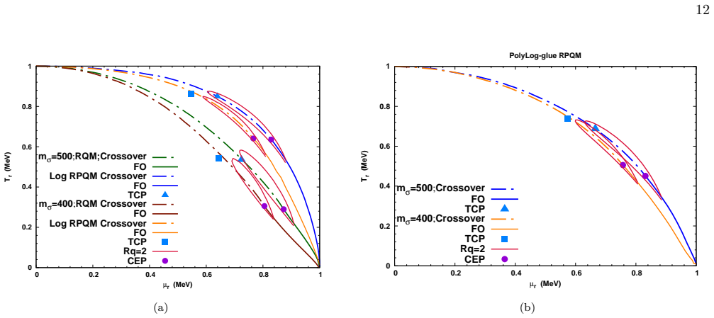
2026-08-03 16:25 UTC pith:6LC7IU4J
load-bearing objection New susceptibility-contour maps for on-shell RQM/RPQM are worth a referee's time, but the central contrast with curvature-mass models rests on one renormalization-scheme choice that gets no sensitivity test. the 1 major comments →
Comparative analysis of critical regions: The renormalized quark-meson model under Polyakov loop, quark back-reaction, and vector interaction effects
The pith
A machine-rendered reading of the paper's core claim, the machinery that carries it, and where it could break.
Core claim
Consistent on-shell renormalization of the 2+1-flavor quark-meson model—counterterms matched to pole masses, scale Λ0 fixed by Eq. (13)—strengthens the 't Hooft coupling, weakens chiral symmetry breaking, and shifts the critical end point to larger μ, lower T than curvature-mass parametrizations. Contours of normalized quark number susceptibility Rq=χq/χq^{free} then envelop the CEP in large, smooth, roughly symmetric regions (Rq=2 spans 50.2 MeV in T, 58.3 MeV in μ for mσ=500 MeV), versus the narrow, pinched contours of QMVT/PQMVT models. For mσ=500 MeV the tricritical point sits inside the Rq=2 contour, so it can influence CEP fluctuations; for mσ=400 MeV it lies outside. Quark back-reacti
What carries the argument
The central object is the on-shell renormalized vacuum effective potential, built by matching MS-scheme counterterms to on-shell pole masses of π, K, η, η′, and σ, with the renormalization scale Λ0 fixed so the vacuum minimum does not shift from the unrenormalized model. The diagnostic is the ratio Rq = χq/χq^{free} of the quark number susceptibility to the free-quark-gas value, drawn as contours (Rq=2, 3, 5) in the μ-T plane. This ratio converts the CEP's divergent susceptibility into a finite-size, experimentally relevant 'critical region' whose shape and extent are compared across model settings.
Load-bearing premise
The load-bearing premise is that the on-shell renormalization condition—fixing the scale Λ0 by Eq. (13) and matching counterterms to pole masses—is the correct and unique way to treat quark vacuum fluctuations; a different scheme would change the size and position of the predicted critical regions.
What would settle it
Calculate the same susceptibility contours with a different, equally plausible renormalization condition (e.g., a different Λ0-fixing condition or matching at a different scale) and check whether the Rq=2 spreads change by more than ~10 MeV; if they do, the claimed 'large, smooth critical region' is an artifact of the scheme. Alternatively, a direct lattice QCD determination of the CEP's location and the phase-boundary curvature at finite density could falsify the RQM/RPQM predictions, which place the CEP near (265,39) MeV for mσ=500 or (243,37) MeV for mσ=400 in the physical-point parametriza
If this is right
- If the on-shell treatment is correct, heavy-ion beam-energy-scan searches should expect a broad, rounded critical region extending tens of MeV in both temperature and chemical potential around the CEP, rather than a thin sliver.
- For mσ=500 MeV, the tricritical point's location inside the Rq=2 contour means the CEP's critical fluctuations inherit tricritical influence, altering the expected scaling of higher-order cumulants.
- The quark back-reaction in the PolyLog-glue Polyakov potential changes the shape of the critical region (rounder, broader in T), so modeling of the deconfinement transition matters for CEP phenomenology.
- The RPQM model's CEP, placed at μ_B≈690–760 MeV and T≈71–95 MeV, lies closer to recent lattice and functional-renormalization-group estimates than the curvature-mass PQMVT model, suggesting the on-shell scheme is the more reliable effective-model benchmark.
Where Pith is reading between the lines
- Editorial note: the abstract announces a vector-interaction analysis in which the CEP and first-order line survive up to g_ω=2.79, but the body text as provided contains no such section; that claim would need its own derivation before being used for compact-star phenomenology.
- The paper itself cautions that two-decimal CEP coordinates reflect numerical binning, not physical precision—a useful reminder that the critical-region extent, not the nominal point, is the robust object.
- A natural test: compute the same Rq contours in a functional renormalization group treatment of the same model to see whether the on-shell scheme's broad regions survive beyond mean-field.
- If the TCP influence is real for mσ=500 MeV, the beam-energy-scan's net-proton cumulant ratios could show non-monotonicity from the combined O(4)-to-Z(2) crossover—an effect the paper maps but does not compute in detail.
Editorial analysis
A structured set of objections, weighed in public.
Referee Report
Summary. The paper computes phase diagrams and quark-number-susceptibility contours (Rq = 2, 3, 5) around the critical end point in a 2+1 flavor quark-meson model with on-shell renormalized quark vacuum fluctuations (RQM), with and without Polyakov loop enhancement (RPQM), for mσ = 400 and 500 MeV. It reports that the consistently on-shell renormalized treatment yields larger, smoother, and more symmetric critical regions than the curvature-mass QMVT/PQMVT scheme of Ref. [118], and that for mσ = 500 MeV the tricritical point lies inside or on the Rq = 2 contour, implying TCP influence on critical fluctuations around the CEP. Light chiral limit phase diagrams are constructed using large-Nc ChPT inputs, and vector-interaction extensions are briefly discussed. The abstract explicitly cautions that the two-decimal CEP coordinates reflect numerical binning, not physical precision.
Significance. If the central claim holds, the paper would establish that the choice of meson-mass renormalization scheme is not a minor technical detail: it qualitatively changes the size and shape of the critical region around the CEP in a widely used effective model. The systematic comparison across QM/RQM/Log-RPQM/PolyLog-glue-RPQM and against Ref. [118] is useful, as is the light-chiral-limit TCP analysis. The paper is unusually candid in the abstract about binning artifacts in reported coordinates. However, no code or data archive is provided, and the central numerical results are imported from the authors' prior on-shell renormalization papers [141,142], so independent verification is currently not possible from the manuscript alone.
major comments (1)
- [Sec. II C and Table III] The light chiral limit results use ChPT inputs from Refs. [61–63] and the parameters are then used to locate the TCP. The paper reports that the TCP lies on/inside the Rq = 2 contour for mσ = 500 MeV but outside for mσ = 400 MeV. This proximity claim is potentially interesting, but it depends on both the on-shell scheme and the ChPT-determined fπ, fK, mη, mη′ in the chiral limit. Given the scheme sensitivity flagged above, the TCP-insertion conclusion should be revisited in the same sensitivity study.
minor comments (4)
- [Section IV] Typo: 'Rq = 2, 35, are drawn' should read 'Rq = 2, 3, 5'. Similar numerical typos appear in other places (e.g., 'mπ = 0, 35' and '(µCEP,T CEP)=(243.12.37.03)').
- [Fig. 4] The axis labels are labeled 'Tr (MeV)' and 'µr (MeV)', but Tr and µr are dimensionless ratios. Please correct the units.
- [Sec. III B] The term 'under no sea mean field approximation' should be 'standard mean field approximation (s-MFA)'. Also, the notation Rq is used for the ratio of susceptibilities, but the text sometimes writes 'Rq = 2, 3 5' with missing comma.
- [Eqs. (41)-(43)] The definition of χq_free as the massless free quark gas value is clear, but the contours of Rq = 2, 3, 5 are not derived from any universality or scaling argument. It would be helpful to state explicitly that these are heuristic measures of critical-region extent, not model-independent quantities.
Circularity Check
No significant circularity: CEP/TCP and Rq contours are computed outputs, not fitted inputs; the on-shell scheme is a stated modeling assumption rather than a self-referential prediction.
full rationale
The paper's parameter fixing is standard and external: at the physical point, m_pi, m_K, M_eta, m_sigma, f_pi, f_K and the Yukawa coupling g determine the QM/RQM couplings (Table II), while the light-chiral-limit inputs follow from large-Nc ChPT with L8, v31 and v02 fixed to reproduce the physical M_eta [63]. The CEP, TCP and Rq=2/3/5 contours are then obtained by minimizing the grand potential and differentiating with respect to mu; none of these outputs is fed back into the parameter determination. Equation (13), which fixes Lambda_0 by requiring that the RQM vacuum minimum does not shift from the QM minimum, is an explicit renormalization-scheme condition imported from the authors' prior papers [141,142]; this is a model assumption whose sensitivity is not tested, but it is not a hidden fit and does not make the critical-region claim equivalent to its inputs. The statement that on-shell pole masses m_eta and m_eta' are reproduced after self-energy corrections is a self-consistency check of the chosen OS scheme, not a prediction derived from the scheme. The heavy reliance on Refs. [63,141,142] is cumulative use of prior peer-reviewed derivations; no uniqueness theorem is invoked to forbid alternatives, and no ansatz is passed off as externally established. Hence no step in the derivation chain reduces by construction to its own input; the scheme-dependence concern belongs to robustness/sensitivity rather than circularity.
Axiom & Free-Parameter Ledger
free parameters (4)
- sigma meson mass m_sigma =
400 and 500 MeV
- Yukawa coupling g =
not stated in visible text
- Polyakov scale T0 (and T_glue^c) =
187 MeV for 2+1 flavors; 270 MeV for pure gauge
- PolyLog-glue temperature mapping coefficient =
0.57
axioms (5)
- domain assumption Mean-field treatment of meson fields: only quark/antiquark thermal and vacuum fluctuations are included; meson fields are treated classically.
- ad hoc to paper On-shell renormalization scheme: pole masses of mesons are the physical masses, and counterterms are matched between MS and on-shell schemes as developed in Refs. [141,142].
- domain assumption Large-N_c U(3) chiral perturbation theory inputs are used to extrapolate f_pi, f_K, m_eta, m_eta' to the light chiral limit (m_pi=0, m_K=496 MeV), with L8, v31, v02 fixed to reproduce M_eta at the physical point.
- domain assumption The logarithmic and PolyLog-glue forms of the Polyakov-loop potential, with the T0(T_glue^c)=187 MeV mapping, faithfully capture confinement-deconfinement and quark back-reaction effects.
- standard math The quark number susceptibility ratio R_q = chi_q / chi_q^free identifies the critical region, with R_q=2,3,5 contours representing enhanced critical fluctuations.
read the original abstract
The critical regions enveloping the critical end point (CEP) in the $\mu$-$T$ plane are mapped by computing the contours of normalized quark number susceptibility within the on shell renormalized 2+1 flavor quark-meson (RQM) and Polyakov loop enhanced renormalized Polyakov quark meson (RPQM) models for $m_\sigma = 400$ and 500 MeV.The apparent precision for the results of CEP coordinates merely reflects numerical binning of two decimal places rather than the effect of including full thermal and vacuum quantum fluctuations. The renormalized 't Hooft coupling c becomes substantially stronger in the RQM model when the meson self energies due to quark loops are computed using the pole masses of mesons and parameters are fixed on shell in Ref [143] after a consistent treatment of quark one loop vacuum fluctuations while the light and strange chiral symmetry breaking strengths also become weaker. We evaluate the impact of these novel features on critical fluctuations. Furthermore, the improved PolyLog glue form of the Polyakov loop potential from Ref [46] is employed to isolate the effects of the quark back reaction on critical fluctuations, and the results are contrasted against back reaction free outcomes obtained using the logarithmic potential. Utilizing inputs from large $N_c$ standard chiral perturbation theory, phase diagrams are also computed in the light chiral limit ($m_\pi = 0$), quantifying the proximity of the tricritical point (TCP) to the CEP. The critical regions from the RQM/RPQM models are compared with those reported in Ref [120], where curvature masses are used for parameter fixing. Phase diagrams incorporating vector interactions in the RQM/RPQM model reveal that the CEP and first-order transition survive up to a robust coupling of $g_\omega = 2.79$, rendering them highly relevant for compact star equations of state and astrophysical phenomenology.
Figures




Reference graph
Works this paper leans on
-
[1]
Cabibbo and G
N. Cabibbo and G. Parisi, Phys.Lett.B 59 ,67-69(1975)
1975
-
[2]
PQMVT model CEP is placed at significantly higher TCEP = 90 MeV whereas the CEP in both the QMVT and PQMVT models gets located at larger chemical po- tentials around 280–285 MeV [ 118]. The PQMVT model contour of a successively decreasing width below its TCEP, has a larger neck like narrow structure because the curvature of the first order transition line b...
-
[3]
Muller, Rep
B. Muller, Rep. Prog. Phys. 58, 611 (1995)
1995
-
[4]
The curvatures of the crossover and first order transition lines in the Fig
Divid- ing the temperature T by the highest temperature T χ c of the chiral crossover transition on the temperature axis at µ = 0, one gets the Tr = T T χ c and when the chemical po- tentialµ is divided by the highest chemical potential µ0 at which first order phase transition on the µ axis occurs at T = 0, one gets the µr = µ µ0 . The curvatures of the cr...
-
[5]
D. H. Rischke, Prog. Part. Nucl. Phys. 52, 197 (2004)
2004
-
[6]
A.Ali Khan et al. Phys. Rev. D 64 , 074510 (2001)
2001
-
[7]
Digal, E
S. Digal, E. Laermann and H. Satz, Eur. Phys. J. C 18 , 583 (2001) . [8]
2001
-
[8]
to the thermal contributions of quarks-antiquarks in the presence of the Polyakov loop potential as the fol- lowing. ΩP QM(T,µ ;x,y, Φ, ¯Φ) = U (x,y ) + Ωq ¯q(T,µ ;x,y, Φ, ¯Φ) (36) The temperature T and chemical potential µ depen- dence of the non-strange condensate x, strange conden- sate y, Φ and ¯Φ are obtained in the RPQM and PQM model by optimizing t...
-
[9]
C. R. Allton, M. Doring, S. Ejiri, S. J. Hands, O. Kaczmarek, F. Karsch, E Laermann and K. Redlich, Phys. Rev. D 71 , 054508 (2005)
2005
-
[10]
in the quark-antiquark contribution to the total effective potential, gets modified by the Polyakov loop potential. ΩT,µ q ¯q (x,y, Φ, ¯Φ) = −2Nc ∑ q ∫ d3p (2π)3T [ lng+ f + lng− f ] .(32) The Ω T,µ q ¯q (x,y, Φ, ¯Φ) = Ω q ¯q(T,µ ;x,y, Φ, ¯Φ) and new g± f being different from their earlier values in the Eq. ( 10), are the following : g+ f = [ 1 + 3Φe−E+ q /T...
-
[11]
L. D. McLerran and B. Svetitsky, Phys. Rev. D 24, 450 (1981) ; B. Svetitsky, Phys. Rep. 132, 1 (1986)
1981
-
[12]
Meyer-Ortmanns, Rev
H. Meyer-Ortmanns, Rev. Mod. Phys. 68, 473 (1996)
1996
-
[13]
Cheng et al., Phys
M. Cheng et al., Phys. Rev. D 77 , 014511 (2008)
2008
-
[14]
is added to the thermal contributions of quarks-antiquarks in the presence of the Polyakov loop potential. ΩRP QM (T,µ ;x,y, Φ, ¯Φ) = Ω RQM vac (x,y ) + Ωq ¯q(T,µ ;x,y, Φ, ¯Φ) (35) When quark one-loop vacuum contribution is dropped in the s-MF A,one gets the PQM model grand thermody- namic potential after adding the meson contribution in Eq. (
-
[15]
Bazavov et al., Phys
A. Bazavov et al., Phys. Rev. D 80, 014504 (2009)
2009
-
[16]
Fodor, S
Z. Fodor, S. D. Katz, and K. K. Szabo, Phys. Lett. B 568 , 73 (2003)
2003
-
[17]
Karsch, Lect
F. Karsch, Lect. Notes Phys. 583, 209 (2002)
2002
-
[18]
Karsch, J
F. Karsch, J. Phys. G 31 , S633 (2005)
2005
-
[19]
Y. Aoki, Z. Fodor, S. D. Katz and K. K. Szabo, Phys. Lett. B 643 , 46 (2006)
2006
-
[20]
Cheng et al., Phys
M. Cheng et al., Phys. Rev. D 74 , 054507 (2006)
2006
-
[21]
Fejos, A
G. Fejos, A. Hosaka, Phys. Rev. D 94, 036005 (2016)
2016
-
[22]
Langelage, S
J. Langelage, S. Lottini, and O. Philipsen, J. High Energy Phys. 02 (2011) 057
2011
-
[23]
Fejos, A
G. Fejos, A. Hosaka, Phys. Rev. D 98, 036009 (2018)
2018
-
[24]
Ejiri et al., Phys
S. Ejiri et al., Phys. Rev. D 80, 094505 (2009)
2009
-
[25]
(27) The summary of the parameters is given in the Table I
are defined as : ai(T ) = a(i) 0 +a(i) 1 ( T0 T ) +a(i) 2 ( T0 T ) 2 1 +a(i) 3 ( T0 T ) +a(i) 4 ( T0 T ) 2 (26) b(T ) = b0 ( T0 T ) b1[ 1 −eb2( T0 T ) b3 ] . (27) The summary of the parameters is given in the Table I. TABLE I. Parameters of the PolyLog Polyakov-loop potential have been taken from the Ref. [ 47]. PolyLog a(2) 0 a(2) 1 a(2) 2 a(2) 3 a(2) 4 2...
-
[26]
M. G. Alford, A. Schmitt and K .Rajagopal, Rev. Mod. Phys. 80, 1455 (2008)
2008
-
[27]
Fukushima, and T
K. Fukushima, and T. Hatsuda, Rep. Prog. Phys. 74, 014001 (2011)
2011
-
[28]
Fejos, Phys
G. Fejos, Phys. Rev. D 92, 036011 (2015)
2015
-
[29]
J. T. Lenaghan, Phys. Rev. D 63 , 037901 (2001)
2001
-
[30]
D 96, 016009 (2017)
Fabian Rennecke, Bernd-Jochen Schaefer, Phys, Rev. D 96, 016009 (2017)
2017
-
[31]
Pedro Costa, M. C. Ruivo, C. A. de Sousa and Yu. L. Kalinovsky, Phys. Rev. D 71 , 116002 (2005)
2005
-
[32]
Fejos, A
G. Fejos, A. Patkos, Phys. Rev. D 105, 096007 (2022)
2022
-
[33]
’t Hooft, Phys
G. ’t Hooft, Phys. Rev. Lett. 37, 8 (1976)
1976
-
[34]
B. J. Schaefer and M. Wagner, Phys. Rev. D 79 , 014018 (2009)
2009
-
[35]
and Eq. ( 36) . ∂ΩRP QM/P QM ∂x = ∂ΩRP QM/P QM ∂y = ∂ΩRP QM/P QM ∂Φ = ∂ΩRP QM/P QM ∂ ¯Φ = 0 (37) The 2+1 flavor RPQM and PQM model phase diagram with Log form and PolyLog-glue form of the Polyakov loop potential, different thermodynamic quantities and critical end point have been calculated and presented in the ref.[ 142]. We will be using the above describ...
-
[36]
Meyer-Ortmanns and B
H. Meyer-Ortmanns and B. J. Schaefer, Phys. Rev. D 53 , 6586 (1996)
1996
-
[37]
J. T. Lenaghan, D. H. Rischke and J. Schaffner-Bielich, Phys. Rev D 62 , 085008 (2000) . J. T. Lenaghan, D. H. Rischke, J. Phys. G 26 , 431 (2000)
2000
-
[38]
Pedro Costa, M. C. Ruivo, C. A. de Sousa and Yu. L. Kalinovsky, AIP Conf. Proc. 775, 173–181 (2005) . 21
2005
-
[39]
Ratti, M
C. Ratti, M. A. Thaler, and W. Weise, Phys. Rev. D 73, 014019 (2006)
2006
-
[40]
Fukushima, Phys
K. Fukushima, Phys. Rev. D 77 , 114028 (2008); 78, 039902(E) (2008)
2008
-
[41]
A. M. Polyakov, Phys. Lett. B 72 , 477 (1978)
1978
-
[42]
Svetitsky and L
B. Svetitsky and L. G. Yaffe, Nucl. Phys. B 210, 423 (1982)
1982
-
[43]
Banks and A
T. Banks and A. Ukawa, Nucl. Phys. B 225, 145 (1983)
1983
-
[44]
R. D. Pisarski, Phys. Rev. D 62 , 111501(R) (2000)
2000
-
[45]
Fukushima, Phys
K. Fukushima, Phys. Lett. B 591, 277 (2004)
2004
-
[46]
Layek, A
B. Layek, A. P. Mishra, A. M. Srivastava and V. K. Tiwari, Phys. Rev. D 73 , 103514 (2006)
2006
-
[47]
P. M. Lo, B. Friman, O. Kaczmarek, K. Redlich, and C. Sasaki, Phys. Rev. D 88 , 074502 (2013)
2013
-
[48]
Roessner, C
S. Roessner, C. Ratti and W. Weise, Phys. Rev. D 75, 034007 (2007)
2007
-
[49]
B. J. Schaefer, J. M. Pawlowski, and J. Wambach, Phys. Rev. D 76 , 074023 (2007)
2007
-
[50]
B. J. Schaefer, M. Wagner, and J. Wambach, Phys. Rev. D 81 , 074013 (2010)
2010
-
[51]
B. J. Schaefer, M. Wagner and J. Wambach, CPOD(2009)017, arXiv:0909.0289
Pith/arXiv arXiv 2009
-
[52]
H. Mao, J. Jin, and M. Huang, J. Phys. G 37 , 035001
-
[53]
U. S. Gupta and V. K. Tiwari, Phys. Rev. D 81 , 054019 (2010)
2010
-
[54]
L. M. Haas, R. Stiele, J. Braun, J. M. Pawlowski and J. Schaffner-Bielich, Phys. Rev. D 87 , 076004 (2013)
2013
-
[55]
Asakawa and K
M. Asakawa and K. Yazaki, Nucl. Phys. A 504 , 668, (1989)
1989
-
[56]
Stiele and J
R. Stiele and J. Schaffner-Bielich, Phys. Rev. D 93 , 094014 (2016)
2016
-
[57]
T. K. Herbst, J. M. Pawlowski, and B.-J. Schaefer, Phys. Lett. B 696, 58 (2011)
2011
-
[58]
T. K. Herbst, J. M. Pawlowski, and B.-J. Schaefer, Phys. Rev. D 88, 014007 (2013)
2013
-
[59]
Bors´ anyi, Z
S. Bors´ anyi, Z. Fodor, C. Hoelbling, S. D. Katz, S. Krieg, C. Ratti, and K. K. Szab´ o, J. High Energy Phys. 09 (2010) 73
2010
-
[60]
Borsanyi, G
S. Borsanyi, G. Endrodi, Z. Fodor, A. Jakovac, S. D. Katz, S. Krieg, C. Ratti and K. K. Szabo, JHEP 11, (2010) 077 . ; S. Borsanyi, Z. Fodor, C. Hoelbling, S. D. Katz, S. Krieg and K. K. Sz- abo, Phys. Lett. B 730 (2014) 99-104
2010
-
[61]
Bazavov et al., Phys
A. Bazavov et al., Phys. Rev. D 85 , 054503 (2012) ; Phys. Rev. D 90, 094503 (2014)
2012
-
[62]
R. D. Pisarski and F. Wilczek, Phys. Rev. D 29, 338 (1984)
1984
-
[63]
V. K. Tiwari, Phys. Rev. D 111, 114014 (2025)
2025
-
[64]
Barducci, R
A. Barducci, R. Casalbuoni, S. De Curtis, R. Gatto, and G. Pettini, Phys. Lett. B 231 , 463 (1989) ; Phys. Rev. D 41 , 1610 (1990)
1989
-
[65]
Berges and K
J. Berges and K. Rajagopal, Nucl. Phys. B 538 , 215 (1999)
1999
-
[66]
Hatta and T
Y. Hatta and T. Ikeda, Phys. Rev. D 67 , 014028 (2003)
2003
-
[67]
Fujii, Phys
H. Fujii, Phys. Rev. D 67 , 094018 (2003)
2003
-
[68]
8 838-844, (2011)
Fukushima, Kenji Physics of Particles and Nuclei Letters. 8 838-844, (2011)
2011
-
[69]
Herrera-Sikl´ ody, J
P. Herrera-Sikl´ ody, J. I. Latorre, P. pascual and J. Taron, Phys. Lett. B 419, 326 (1998)
1998
-
[70]
Escribano, F
R. Escribano, F. S. Ling, M. H. G. Tytgat, Phys. Rev. D 62, 056004 (2000)
2000
-
[71]
G.Odyniec; RHIC Beam Energy Scan Program: Phase I and II, PoS CPOD 2013, 043(2013) and PoS CORFU2018 151 (2019)
2013
-
[72]
V. K. Tiwari, Phys. Rev. D 112, 054046 (2025)
2025
-
[73]
D. T. Son and M. A. Stephanov, Phys. Rev. D 70 , 056001 (2004) ; Y. Aoki, G. Androdi, Z. Fodor, S. D. Katz, and K. K. Szabo, Nature (London) 443, 675 (2006) ; S. Gupta,X. Luo, B. Mohanty, H. G. Ritter, and N. Xu, Science 332,1525 (2011)
2004
-
[74]
M. A. Stephanov, K. Rajagopal, and E. V. Shuryak, Phys.Rev. D 60, 114028 (1999) ; Phys. Rev. Lett. 81, 4816 (1998)
1999
-
[75]
Berdnikov and K
B. Berdnikov and K. Rajagopal, Phys. Rev. D 61 , 105017 (2000)
2000
-
[76]
Jeon and V
S. Jeon and V. Koch, Phys. Rev. Lett. 85, 2076 (2000)
2076
-
[77]
Ejiri, F
S. Ejiri, F. Karsch, and K. Redlich, Phys. Lett. B 633 , 275 (2006)
2006
-
[78]
Adams et al
J. Adams et al. (STAR Collaboration), Nucl. Phys. A 757, 102 (2005) ; M. Ag- garwal et al. (STAR Collaboration), Phys. Rev. Lett. 105, 022302 (2010)
2005
-
[79]
Mohanty, Nucl
B. Mohanty, Nucl. Phys. A 830, 899c (2009) .; X. Luo, B. Mohanty, H. G. Ritter, and N. Xu, Phys. At. Nucl. 75, 676 (2012)
2009
-
[80]
Liu et al
C. Liu et al. 13th Int. Particle Acc. Conf. WEPOPT032
discussion (0)
Sign in with ORCID, Apple, or X to comment. Anyone can read and Pith papers without signing in.